Matplotlib and the Dark Sky API
October 19, 2012 at 10:05 PM by Dr. Drang
Last night, Than Tibbetts responded to my Check the Weather review with this:
@drdrang Why not hook your own script up to the Dark Sky API?
— Than Tibbetts (@thanland) Thu Oct 18 2012 9:35 PM CDT
Which, of course, led me to spend a couple of hours playing around with the Dark Sky API. Nothing of any significance came of it, but it gave me more practice with matplotlib.
The people who make the hyperlocal weather app, Dark Sky, have opened up their API so regular mortals can access the app’s short-term rainfall forecast. As it happens, there’s more information in the API than is presented in the Dark Sky app itselft. Take a look at the documentation for the forecast call and you’ll see that the call returns this piece of info:
error—The 3-sigma error of the intensity value, conditional on precipitation. In other words, if there is precipitation, then 99.7% of the time the intensity value will be between intensity ± error.
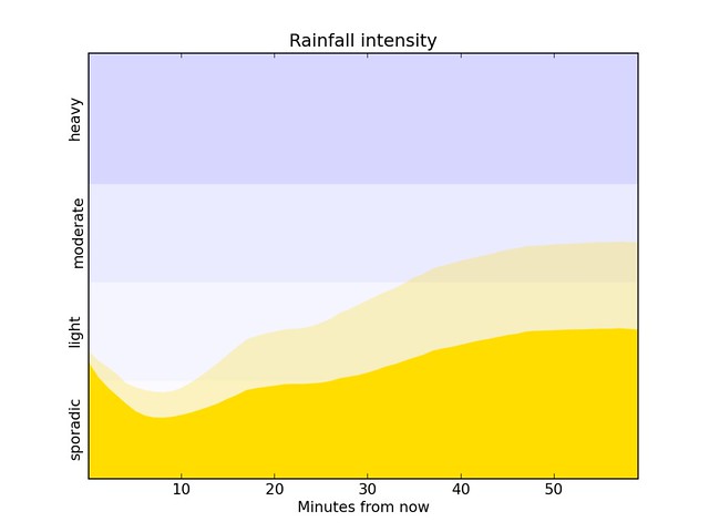
The rain prediction plot in Dark Sky shows only the expected rainfall intensity; one could take this error value and also plot the uncertainty in the prediction. So that’s what I did. Here’s one plot, with the bright yellow, representing the expected rainfall intensity, plotted more or less the way Dark Sky does; and with the duller, see-through yellow, representing the 95th percentile value (assuming a normal distribution), plotted above it.
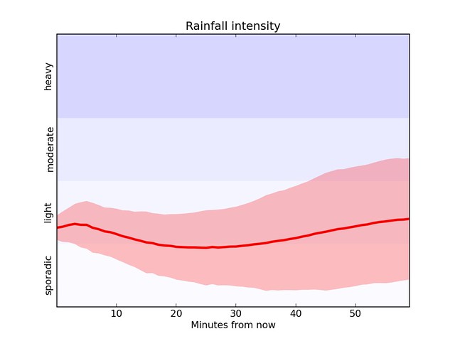
Here’s another, in which the expected rainfall is plotted as a line, and the 95% range is plotted as a band surrounding it.
This one is very much like the interquartile range plots I did in my last matplotlib post, but this one shows the middle 95% instead of the middle 50%.
The script that produced both of these plots is fairly short and easy to understand.
python:
 1:  #!/usr/bin/python
 2:
 3:  from __future__ import division
 4:  import json
 5:  import urllib
 6:  from os import environ
 7:  from sys import exit, argv
 8:  import scipy.stats as stats
 9:  import matplotlib.pyplot as plt
10:
11:  # The probability and number of standard deviations
12:  # associated with the upper and lower bounds.
13:  pUpper = .95
14:  pLower = .025
15:  nUpper = stats.norm.ppf(pUpper)
16:  nLower = stats.norm.ppf(pLower)
17:
18:  # Get the latitude and longitude from the command line
19:  # or use default values from downtown Naperville.
20:  try:
21:    lat = argv[1]
22:    lon = argv[2]
23:  except IndexError:
24:    lat = 41.772903
25:    lon = -88.150392
26:
27:  # Get my API key and construct the URL
28:  try:
29:    with open(environ['HOME'] + '/.darksky') as rcfile:
30:      for line in rcfile:
31:        k, v = line.split(':')
32:        if k.strip() == 'APIkey':
33:          APIkey = v.strip()
34:      dsURL = 'https://api.darkskyapp.com/v1/forecast/%s/%s,%s' % (APIkey, lat, lon)
35:  except (IOError, NameError):
36:    print "Failed to get API key"
37:    exit()
38:
39:  # Get the data from Dark Sky.
40:  try:
41:    jsonString = urllib.urlopen(dsURL).read()
42:    weather = json.loads(jsonString)
43:  except (IOError, ValueError):
44:    print "Connection failure to %s" % dsURL
45:    exit()
46:
47:  # Pluck out the hourly rain forecast information.
48:  startTime = weather['hourPrecipitation'][0]['time']
49:  intensity = [ x['intensity'] for x in weather['hourPrecipitation'] ]
50:  upper = [ min(x['intensity'] + x['error']/3*nUpper, 75) for x in weather['hourPrecipitation'] ]
51:  lower = [ max(x['intensity'] + x['error']/3*nLower, 0) for x in weather['hourPrecipitation'] ]
52:  time = [ (x['time'] - startTime)/60 for x in weather['hourPrecipitation'] ]
53:
54:  # Plot the intensity ranges.
55:  plt.fill_between([0, 59], [15, 15], [0, 0], color='#0000ff', alpha=.02, linewidth=0)
56:  plt.fill_between([0, 59], [30, 30], [15, 15], color='#0000ff', alpha=.04, linewidth=0)
57:  plt.fill_between([0, 59], [45, 45], [30, 30], color='#0000ff', alpha=.08, linewidth=0)
58:  plt.fill_between([0, 59], [75, 75], [45, 45], color='#0000ff', alpha=.16, linewidth=0)
59:
60:  # Plot the values.
61:  plt.fill_between(time, intensity, color='#ffdd00', linewidth=2)
62:  plt.fill_between(time, upper, intensity, color='#ffdd00', alpha=.25, linewidth=0)
63:  # plt.plot(time, intensity, color='#ff0000', linewidth=3)
64:  # plt.fill_between(time, upper, lower, color='#ff0000', alpha=.25, linewidth=0)
65:  plt.axis([0, 59, 0, 65])
66:  plt.xticks([10, 20, 30, 40, 50])
67:  plt.yticks([7.5, 22.5, 37.5, 55], ['sporadic', 'light', 'moderate', 'heavy'], rotation=90)
68:  plt.tick_params('y', length=0)
69:  plt.xlabel('Minutes from now')
70:  plt.title('Rainfall intensity')
71:
72:  plt.savefig('ds-rain-1.png', dpi=160)
73:  # plt.savefig('ds-rain-2.png', dpi=160)
Lines 11-16 use the scipy.stats module to determine how wide, in standard deviations, the band will be. They’re currently set to generate the first plot, where only the upper bound, at the 95th percentile, was plotted. For the second plot, Line 13 was changed to
pUpper = 0.975
Lines 18-25 set the location for which the prediction is made. The latitude and longitude are expected to be the first and second arguments on the command line. If either or both are missing, a default location (the Apple Store in downtown Naperville, Illinois) is used.
Lines 27-37 gather my Dark Sky API key from a dotfile in my home directory (~/.darksky) and use it to construct the URL that makes the call to Dark Sky’s forecast method. The contents of the dotfile look like this:
APIkey: 123456789abcdefg
If the dotfile isn’t present or it doesn’t contain data in the right form, the script quits with an error message.
It’s easy to get a Dark Sky API key. Just give them your email address and a password and you’ll get a key. No need to tell them what you’re going to do with it. They do limit you to 10,000 calls per day before they either cut you off or start charging you (they can only charge you if they have your credit card on file). That’s a huge number for personal use, and I can’t imagine anyone blowing through it (unless you write a script with a loop that goes rogue).
Lines 39-45 collect the data from Dark Sky and decode it into a data structure. Like most web services nowadays, Dark Sky uses JSON to pass information around, and like most scripting languages, Python has a library for handling JSON. If something goes wrong in the download or the decoding, the script quits with an error message.
I should mention here that there is a Python module for Dark Sky on GitHub that I could have used. If I were going to do a lot with the Dark Sky API, I probably would use it; but because it depends on a handful of nonstandard modules I’d have to install, and I was only making one call to the API, it didn’t seem worth the effort for this script.
Lines 47-52 run through the data structure and pull out the time, intensity, and error values of the hourPrecipitation list. We use the intensity value directly. The error value is used, along with intensity and the upper and lower limit numbers calculated in Lines 11-16, to set the upper and lower band values. The time, which is the number of seconds since the start of the Unix epoch, is converted into the number of minutes from now associated with each predicted intensity value.
There’s a brief discussion in the forecast documentation on the meaning of the intensity value. For our purposes, it’s sufficient to say that it’s a number between 0 and 75 and is interpreted by Dark Sky this way:
| Numerical | Descriptive |
|---|---|
| < 15 | sporadic |
| 15-30 | light |
| 30-45 | moderate |
| > 45 | heavy |
Lines 54-58 use these ranges to create a shaded background for the plot. The intensity (ha ha) of the blue was set for each band by altering the alpha value.
Lines 61-64 plot the data. The uncommented lines generate the first plot, the commented lines (when uncommented) generate the second plot.
Lines 65-70 decorate the axes. I put the descriptive labels along the y-axis at the center of each range and avoiding having tick marks appear by setting their length to zero. Note also that although the rainfall intensity can go up to 75, I set the upper limit of the plot to 65. From what I’ve read, a value above 65 means the kind of storm where you should be in a bunker with your head between your knees, not dicking around with Dark Sky.
Lines 72-73 save the plot to a PNG file that’s 1280×960 pixels. The standard plot size is 8″×6″, regardless of the format, and the bitmapped formats use the dpi setting to set the size in pixels (1280 = 8 × 160). As before, these lines are currently set to produce the first plot; switching the comments produces the second.
As in my baseball posts, my main interest here was to get more experience with matplotlib. What did I learn?
- The
matplotlib.pyplotsubmodule is the one I should be using. It has a Gnuplot-like command structure that fits the way I think. - Colors can be set using hex codes just like the ones used in CSS. You’re not limited to the eight built-in colors that the example plots at matplotlib.org always use.
- The tickmark size can be adjusted without recourse to the object-oriented submodules.
- There’s no need to generate NumPy arrays using matplotlib. Plain ol’ Python lists work just fine because matplotlib does the conversion internally. This saves typing.
Update 10/25/12
Jay Hickey adapted some of this code and made a GeekTool geeklet to display the DarkSky short term precipitation chart on his Desktop, a great idea that I’ll probably steal to add to my NerdTool weather layout.


