And now it’s all this

I just said what I said and it was wrong
Or was taken wrong

Next post Previous post

Transforming section properties and principal directions

January 25, 2018 at 8:26 PM by Dr. Drang

The Python section module has one last function we haven’t covered: the determination of the principal moments of inertia and the axes associated with them. We’ll start by looking at how the moments and products of inertia change with our choice of axes.

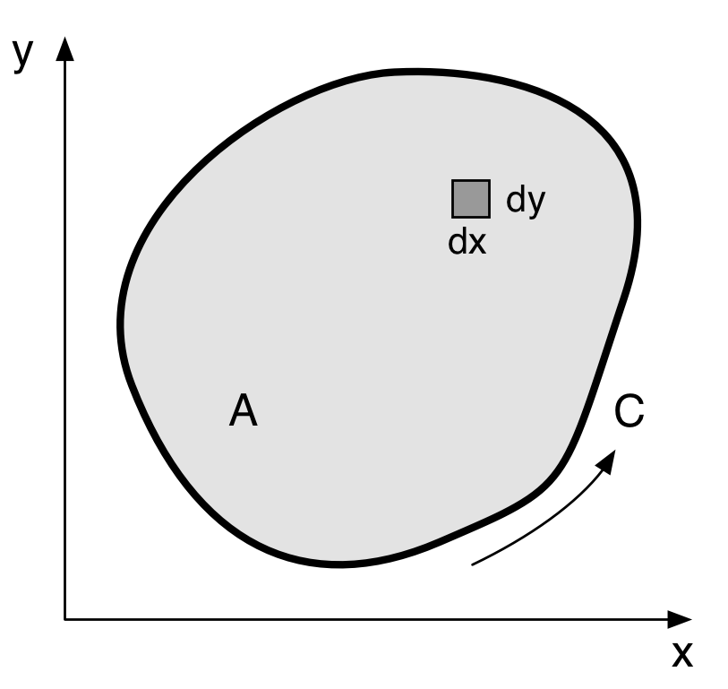
The formula for area,

$$A=\underset{A}{\iint }dxdy$$

will give the same answer regardless of where we put the origin of the $x\text{-}y$ coordinate system or how we orient them. You can see this if you think of the area as being the sum of all the little $dxdy$ squares in the cross-section.

The formulas for the location of the centroid,

$$x_c=\underset{A}{\iint }xdxdy$$ $$y_c=\underset{A}{\iint }ydxdy$$

will give different answers for different positions and orientations of the $x$ and $y$ axes, but those answers will all correspond to same physical point of the cross-section.

The moments and product of inertia as we defined them, relative to the centroid,

$$I_{xx}=\underset{A}{\iint }(y-y_c{)}^{2}dxdy$$ $$I_{yy}=\underset{A}{\iint }(x-x_c{)}^{2}dxdy$$ $$I_{xy}=\underset{A}{\iint }(y-y_c)(x-x_c)dxdy$$

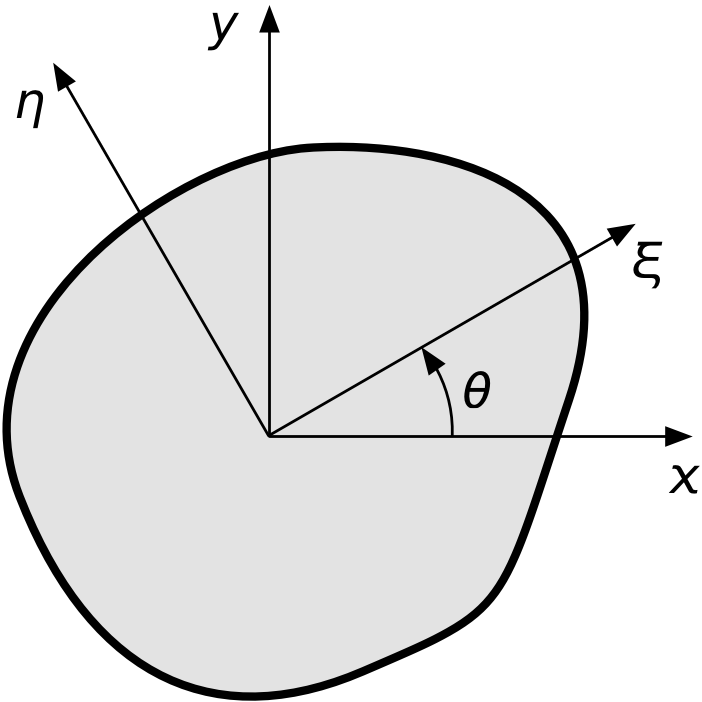
do not depend on the position of the $x\text{-}y$ origin (because $x-x_c$ and $y-y_c$ measure the horizontal and vertical distances away from the centroid, which is the same for any origin), but do depend on the orientation of the axes. We’ll show how this works by putting the origin at the centroid (which simplifies the math but does not make the results any less general) and comparing the moments and product of inertia for two coordinate systems, one of which is rotated relative to the other.

Note that $\theta$ is the angle from the $x$ axis to the $\xi$ axis and is positive in the counterclockwise direction.¹

Because our origin is at the centroid, $x_c=y_c={\xi }_c={\eta }_c=0$, and we can write the equations for the moments and products of inertia in a more compact form:

In the $x\text{-}y$ system,

$$I_{xx}=\underset{A}{\iint }{y}^{2}dxdy$$ $$I_{yy}=\underset{A}{\iint }{x}^{2}dxdy$$ $$I_{xy}=\underset{A}{\iint }xydxdy$$

and in the $\xi \text{-}\eta$ system,

$$I_{\xi \xi }=\underset{A}{\iint }{\eta }^{2}d\xi d\eta$$ $$I_{\eta \eta }=\underset{A}{\iint }{\xi }^{2}d\xi d\eta$$ $$I_{\xi \eta }=\underset{A}{\iint }\xi \eta d\xi d\eta$$

We can go back and forth between the two coordinate systems by noting that

$$\xi =x\cos \theta +y\sin \theta$$ $$\eta =-x\sin \theta +y\cos \theta$$

Thus,

$$I_{\xi \xi }=\underset{A}{\iint }(x^2{\sin }^2\theta -2xy\sin \theta \cos \theta +y^2{\cos }^2\theta )dxdy$$ $$I_{\eta \eta }=\underset{A}{\iint }(x^2{\cos }^2\theta +2xy\sin \theta \cos \theta +y^2{\sin }^2\theta )dxdy$$ $$I_{\xi \eta }=\underset{A}{\iint }((y^2-x^2)\sin \theta \cos \theta +xy({\cos }^2\theta -{\sin }^2\theta ))dxdy$$

The $\theta$ terms can come out of the integrals, leaving us with

$$I_{\xi \xi }={\sin }^2\theta \underset{A}{\iint }{x}^{2}dxdy-2\sin \theta \cos \theta \underset{A}{\iint }xydxdy+{\cos }^2\theta \underset{A}{\iint }{y}^{2}dxdy$$

or

$$I_{\xi \xi }=I_{xx}{\cos }^2\theta +I_{yy}{\sin }^2\theta -2I_{xy}\sin \theta \cos \theta$$

Similarly,

$$I_{\eta \eta }=I_{xx}{\sin }^2\theta +I_{yy}{\cos }^2\theta +2I_{xy}\sin \theta \cos \theta$$ $$I_{\xi \eta }=(I_{xx}-I_{yy})\sin \theta \cos \theta +I_{xy}({\cos }^2\theta -{\sin }^2\theta )$$

So far, this is just a bunch of algebra that could’ve been done quickly in SymPy. Now it’s time to start thinking.

Looking at the expression for $I_{\xi \eta }$, you might notice that each term includes parts from the double angle formulas. So we can rewrite it this way:

$$I_{\xi \eta }=\frac{1}{2}(I_{xx}-I_{yy})\sin 2\theta +I_{xy}\cos 2\theta$$

Note that $I_{\xi \eta }=0$ when

$$(I_{yy}-I_{xx})\sin 2\theta =2I_{xy}\cos 2\theta$$

or

$$\tan 2\theta =\frac{2I_{xy}}{I_{yy}-I_{xx}}$$

Because the tangent function repeats itself every 180°, this expression can be solved with an infinite number of values of $\theta$ that are 90° apart from one another. These orientations all look basically the same, except the $\xi$ and $\eta$ axes swap positions and flip around. For each of them, $I_{\xi \eta }=0$.

Since we’ve written the expression for $I_{\xi \eta }$ in terms of $2\theta$, lets’s do the same for $I_{\xi \xi }$ and $I_{\eta \eta }$. We start by recognizing the double angle formula for sine in each equation:

$$I_{\xi \xi }=I_{xx}{\cos }^2\theta +I_{yy}{\sin }^2\theta -I_{xy}\sin 2\theta$$ $$I_{\eta \eta }=I_{xx}{\sin }^2\theta +I_{yy}{\cos }^2\theta +I_{xy}\sin 2\theta$$

Then we use the thoroughly non-obvious identity,²

$$A{\cos }^2\theta +B{\sin }^2\theta =\frac{A+B}{2}({\cos }^2\theta +{\sin }^2\theta )+\frac{A-B}{2}({\cos }^2\theta -{\sin }^2\theta )$$

and use the usual trig identities to get

$$A{\cos }^2\theta +B{\sin }^2\theta =\frac{A+B}{2}+\frac{A-B}{2}\cos 2\theta$$

Therefore,³

$$I_{\xi \xi }=\frac{I_{xx}+I_{yy}}{2}-\frac{I_{yy}-I_{xx}}{2}\cos 2\theta -I_{xy}\sin 2\theta$$

and

$$I_{\eta \eta }=\frac{I_{xx}+I_{yy}}{2}+\frac{I_{yy}-I_{xx}}{2}\cos 2\theta +I_{xy}\sin 2\theta$$

Now let’s look at how these moments of inertia change with $\theta$. Suppose we wanted to find the $\theta$ that maximized (or minimized) the value of $I_{\xi \xi }$? We’d take the derivative of the expression for $I_{\xi \xi }$ and set it to zero:

$$\frac{d{I}_{\xi \xi }}{d\theta }=(I_{yy}-I_{xx})\sin 2\theta -2I_{xy}\cos 2\theta =0$$

This should look familiar. It’s solution is

$$\tan 2\theta =\frac{2I_{xy}}{I_{yy}-I_{xx}}$$

the same thing we got setting $I_{\xi \eta }=0$. And if we took the derivative of $I_{\eta \eta }$ with respect to $\theta$ and set it to zero to find the maxima and minima of $I_{\eta \eta }$, we’d get the same thing.

These orientations of the axes are known as the principal directions of the cross-section. They give us both a product of inertia of zero and the largest and smallest values of the moments of inertia. (If $I_{\xi \xi }$ is at a maximum, then $I_{\eta \eta }$ is at a minimum, and vice versa.)

The largest and smallest moments of inertia are commonly called $I_1$ and $I_2$, respectively. They can be calculated by substituting our solution for $\theta$ back into the expressions for $I_{\xi \xi }$ and $I_{\eta \eta }$, but there’s some messy math along the way. It’s easier to recognize that the maximum and minimum moments of inertia are determined entirely by the second and third terms of $I_{\xi \xi }$ and $I_{\eta \eta }$, which are in the form

$$A\cos \alpha +B\sin \alpha$$

This expression can be thought of as the horizontal projection of a pair of vectors, one of length $A$ at an angle $\alpha$ to the horizontal and the other of length $B$ at right angles to $A$.

The largest value of this expression will come when the hypotenuse of the triangle, $\sqrt{A^2+B^2}$, is itself horizontal and pointing to the right. The algebraically smallest value will come when the hypotenuse is horizontal and pointing to the left.

Applying this idea to our expressions for $I_{\xi \xi }$ and $I_{\eta \eta }$, the larger principal moment of inertia will be

$$I_1=\frac{I_{xx}+I_{yy}}{2}+\sqrt{{\left(\frac{I_{yy}-I_{xx}}{2}\right)}^2+I_{xy}^2}$$

and the smaller will be

$$I_2=\frac{I_{xx}+I_{yy}}{2}-\sqrt{{\left(\frac{I_{yy}-I_{xx}}{2}\right)}^2+I_{xy}^2}$$

The axis associated with the larger principal moment of inertia is called the major principal axis and the axis associated with the smaller principal moment of inertia is called the minor principal axis. These are sometimes called the strong and weak axes, respectively. Whatever you call them, they’ll be 90° apart.

Now let’s look at the principal function from the section module and see how these formulas were used.

python:
def principal(Ixx, Iyy, Ixy):
  'Principal moments of inertia and orientation.'

  avg = (Ixx + Iyy)/2
  diff = (Ixx - Iyy)/2      # signed
  I1 = avg + sqrt(diff**2 + Ixy**2)
  I2 = avg - sqrt(diff**2 + Ixy**2)
  theta = atan2(-Ixy, diff)/2
  return I1, I2, theta

Looks like I was careless with the $(I_{yy}-I_{xx})$ term and got it backward in the expression for diff, doesn’t it? Also, there seems to be a stray negative sign in the expression for theta. But the principal function does work despite these apparent errors. What we’re running into is the sometimes vexing difference between math and computation.

First, in the formulas for $I_1$ and $I_2$, the diff term gets squared, so flipping its sign doesn’t matter. Second, the numerical calculation of the arctangent isn’t as straightforward as you might think.

There are two arctangent functions in Python’s math library (and in the libraries of many languages):

• atan takes a single argument and returns a result between $-\pi /2$ and $\pi /2$ (-90° and 90°, but in radians instead of degrees).
• atan2 takes two arguments, the $y$ and $x$ components of a vector directed out from the origin at the angle of interest, and returns a result between $-\pi$ and $\pi$ (-180° and 180°), depending on which quadrant the vector points toward.

We can’t use atan in our code because it isn’t robust for some inputs. If we tried

python:
theta = atan(2*Ixy/(Iyy - Ixx))/2

as our formula suggests, we’d get divide-by-zero errors whenever $I_{xx}=I_{yy}$. We can’t have that because there are real cross sections of practical importance for which that’s the case. Any equal-legged angle, for example.

But atan2 can be a problem, too, because we need to distinguish between the major and minor principal axes. In particular, I decided that theta should be the angle between the $x$ axis and the major principal axis. Using atan2 directly from the formula like this

python:
theta = atan2(2*Ixy, Iyy - Ixx)/2

can return an angle 90° away from what we want.

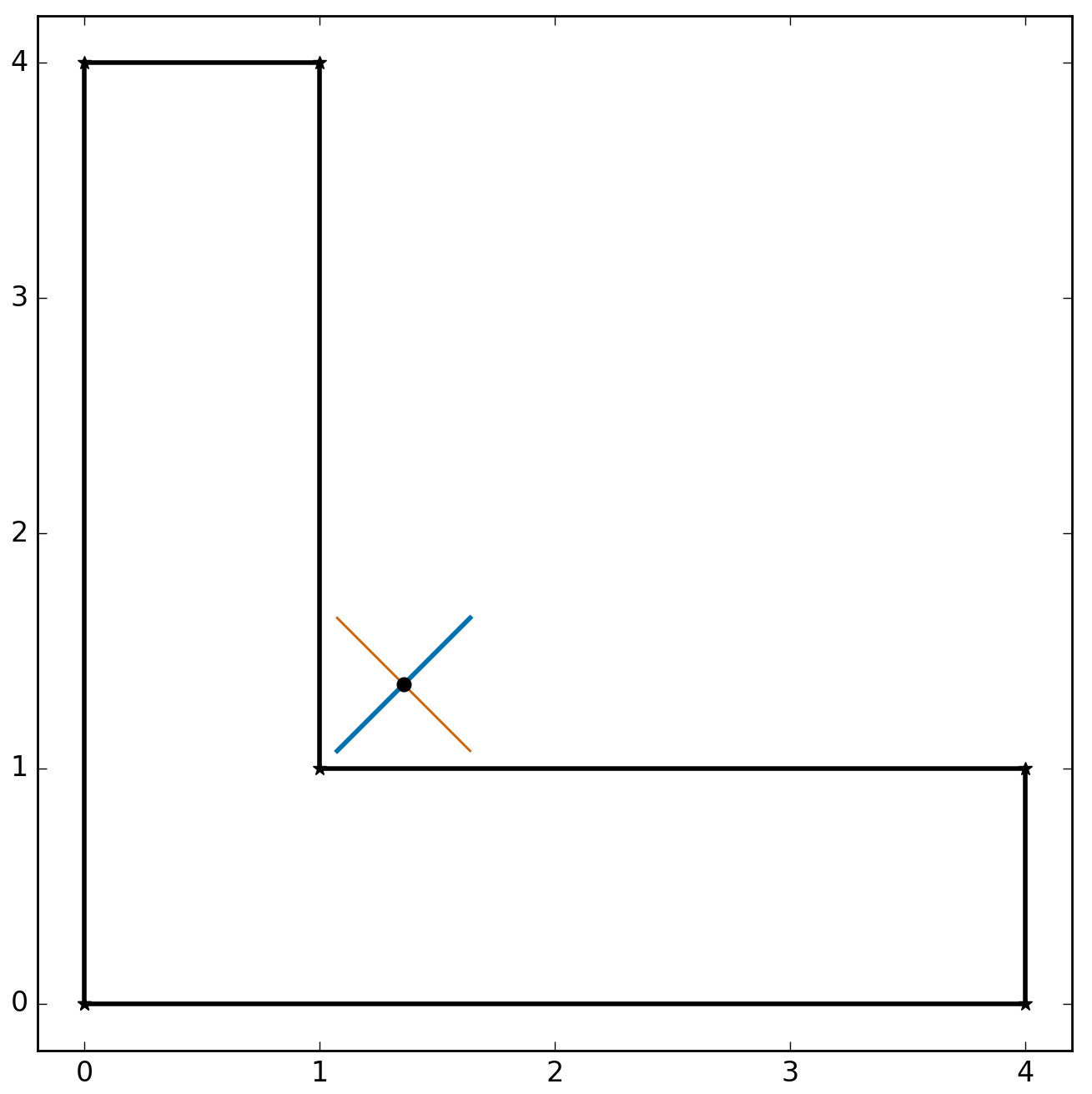
Using the inertia function developed earlier, the moments and product of inertia of the equal-legged angle we just looked at are

Ixx = 9.4405
Iyy = 9.4405
Ixy = -5.1429

Plopping these numbers into the naive formula above, we get

theta = -0.7854

or -45°. This is the angle from the $x$ axis to the weak axis, not the strong axis. The correct answer is 45°, just like the blue line in the figure.

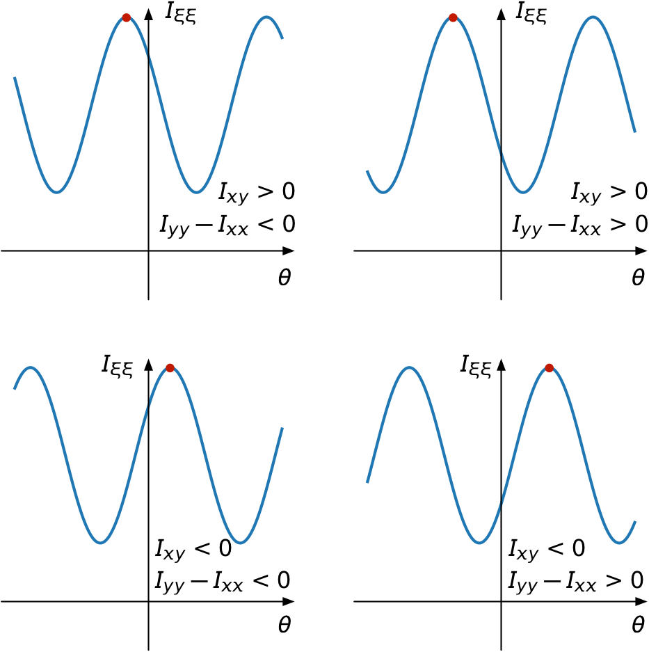
To figure out a way around this problem, let’s plot $I_{\xi \xi }$ for the four cases of interest:

1. $I_{xy}>0\text{and}{I}_{yy}>I_{xx}$

This will let us see what we need for all four quadrants of the atan2 function.

In each of the subplots, successive peaks and valleys of $I_{\xi \xi }$ are 90° apart.

We’re looking for the maximum values of $I_{\xi \xi }$ that are closest to $\theta =0$, which I’ve marked with the red dots. That means

1. When $I_{xy}>0\text{and}{I}_{yy}>I_{xx}$ (upper right), we want the negative $\theta$ with an absolute value greater than 45°.
2. When (upper left), we want the negative $\theta$ with an absolute value less than 45°.
3. When (lower left), we want the positive $\theta$ with an absolute value less than 45°.
4. When (lower right), we want the positive $\theta$ with an absolute value greater than 45°.

The invocation of atan2 that gives us all of these is

python:
theta = atan2(-2*Ixy, Ixx - Iyy)/2

which we can visualize this way, where the curved arrows represent the angle $2\theta$ for each type of result:

By flipping the signs of both arguments of atan2, we get the sign and magnitude of theta we’re looking for. Note that the expression used in the principal function,

python:
theta = atan2(-Ixy, diff)/2

is equivalent to

python:
theta =  atan2(-2*Ixy, Ixx - Iyy)/2

because of the way we defined diff. And by flipping the signs of both the numerator and denominator, we’re not changing the quotient or the definition of $\theta$. We’re just choosing which solution of

$$\tan 2\theta =\frac{2I_{xy}}{I_{yy}-I_{xx}}$$

is the most useful.

If you’re mathematically inclined, you may recognize the rotation of axes as a tensor transformation and the determination of principal moments of inertia and principal directions as a eigenvalue/eigenvector problem. But writing principal in those terms would have required me to use more libraries than just math. The formulas in principal are simple, even if their derivation can take us all over the map.

Now that we’ve figured out how principal works, what good is it? It can be shown⁴ that when the loads on a beam are aligned with one of the principal directions, the beam will bend in that direction only. If the loading is not aligned with a principal direction, the beam will bend both in the direction of the load and in a direction perpendicular to it.

For example, if we were using the equal-legged angle above as a beam and hung a vertical downward load off of it, it would bend both downward and to the left. Not the most intuitively obvious result, but true nonetheless.

Everyone who takes an advanced strength of materials class learns the formulas for the principal moments of inertia and their directions, but there’s usually a bit of hand waving to make the math go faster. And, because the strong and weak directions are typically easy to determine by inspection, the details of picking out the correct arctangent value aren’t discussed. But there’s a richness to even the simplest mechanics, I enjoy exploring it. And since computers can’t figure things out by inspection, you can’t gloss over the details when writing a program.

Next post Previous post

Site search

Meta

• drdrang at leancrew
• Blog archive
• RSS feed
• JSON feed
• Mastodon
• GitHub repositories

Recent posts

Credits

This work is licensed under a Creative Commons Attribution-Share Alike 3.0 Unported License.

© 2005–2023, Dr. Drang