And now it’s all this

I just said what I said and it was wrong
Or was taken wrong

Next post Previous post

Swings and roundabouts

February 13, 2023 at 10:09 AM by Dr. Drang

I found Matt Parker’s recent video a bit confusing, and I’d like to talk about it. According to the title, it’s about the Runge phenomenon, and while it certainty covers that topic, it starts out pretty far away and takes a sudden swing.¹

The video starts with a formula that Flat-Earthers apparently love: an estimate of how much the horizon should drop with distance. The formula is

$$h=8d^2$$

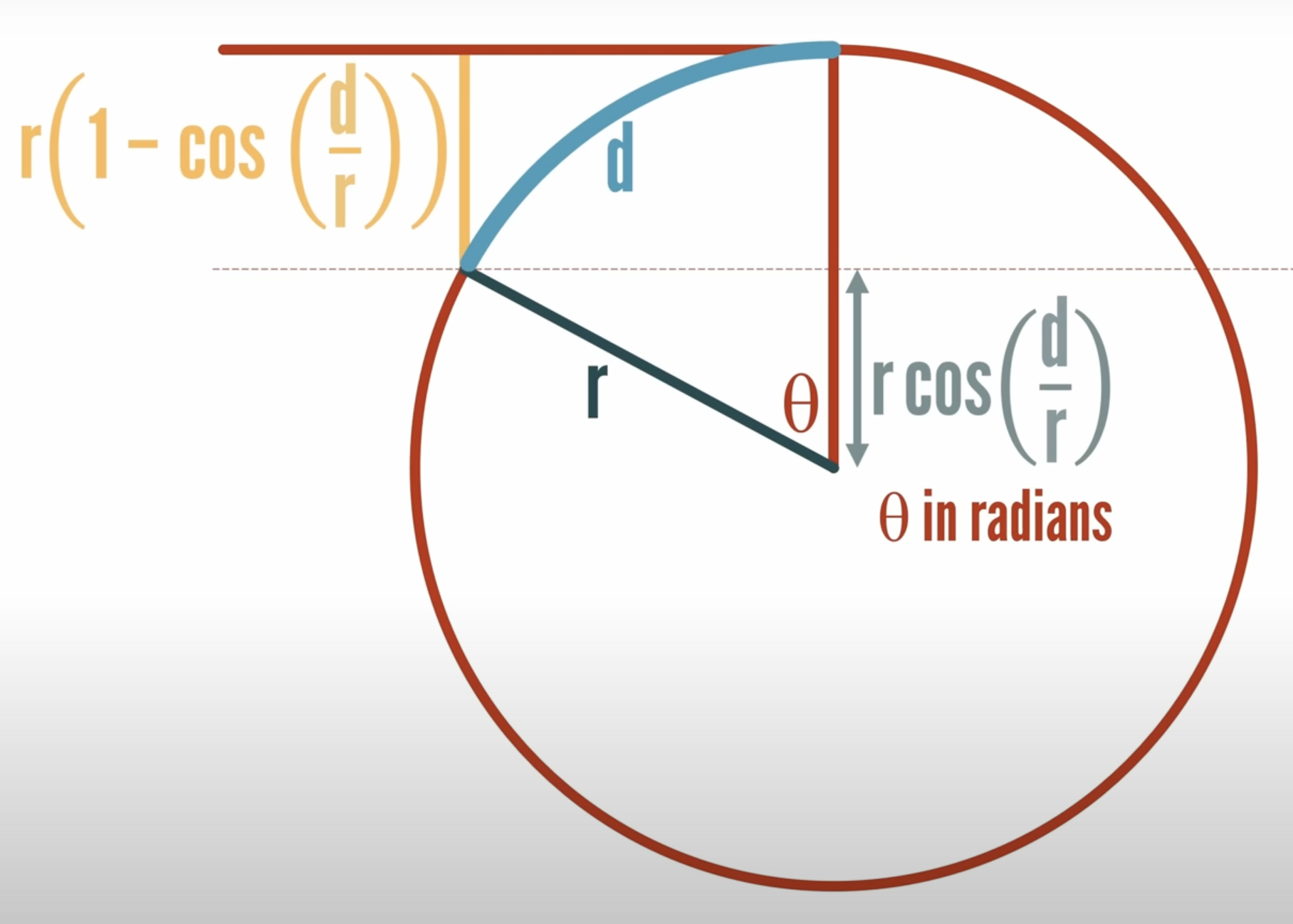
where the horizon drop $h$ is measured in inches and the distance $d$ is measured in miles. Matt wonders where this formula comes from and puts up this figure to work out the real formula

We will, as Matt does, ignore some physical realities and follow the Flat-Earther line of logic without question. From the diagram, it’s clear that the true formula for the horizon drop is

$$h=r(1-\cos \frac{d}{r})$$

At this point, I had forgotten that the video was supposed to be about the Runge phenomenon and expected Matt to do some small-angle approximations and unit conversions to get from this formula to the parabola approximation above. But he doesn’t.

Instead, Matt hauls out a spreadsheet, compares the true formula to the approximate one for several values of $d$, and finds that they’re quite close. This is all very well and good, but it doesn’t explain why the approximate formula works as nicely as it does.

We’re now about seven minutes into the video, and Matt takes what I consider to be a hard left turn to talk about fitting polynomials to other curves by matching them at a set of points. This has nothing to do with how the horizon approximation was derived, but it does lead us to the Runge phenomenon.²

We are, I guess, supposed to think the horizon approximation was derived by fitting a parabola to three points on the real curve, but that’s not how it’s done. Let’s follow the path I thought Matt was going down.

The Taylor series for cosine, expanding about zero,³ is

$$1-\frac{{\theta }^2}{2}+\frac{{\theta }^4}{24}+O\left({\theta }^5\right)$$

When the angle is small, we can truncate this at the squared term. Therefore,

$$1-\cos \theta \approx 1-(1-\frac{{\theta }^2}{2})=\frac{{\theta }^2}{2}$$

Will the angle be small for the horizon problem? Yes. The angle, in radians, is

$$\theta =\frac{d}{r}$$

and for all practical applications, $d$ will be much less than $r$. Therefore, the approximate horizon drop will be

$$h\approx r\left[\frac{1}{2}{\left(\frac{d}{r}\right)}^2\right]=\frac{1}{2}\frac{d^2}{r}$$

This formula works well when $h$, $d$, and $r$ are in consistent units, but the Flat-Earther formula doesn’t use consistent units. To get a formula that accounts for the known radius of the Earth (3958.8 miles) and converts $h$ from miles to inches, we do the following:

$$h\approx \frac{1}{2}\frac{d^2}{3958.8\mathrm{m}\mathrm{i}\mathrm{l}\mathrm{e}\mathrm{s}}\left(\frac{5280\mathrm{f}\mathrm{t}}{1\mathrm{m}\mathrm{i}\mathrm{l}\mathrm{e}\mathrm{s}}\right)\left(\frac{12\mathrm{i}\mathrm{n}}{1\mathrm{f}\mathrm{t}}\right)=\left(8.0024\mathrm{i}\mathrm{n}\mathrm{·}\mathrm{m}\mathrm{i}\mathrm{l}\mathrm{e}{\mathrm{s}}^{-2}\right)d^2$$

And we can round that 8.0024 down to 8 with no error of any consequence.

So we see that the 8 in the approximate formula is not a pure number; it’s a consequence of the units we chose for $d$ and $h$. This kind of formula, in which certain units are bound up in the coefficients, used to be fairly common in engineering texts. I’ve seen it often in old⁴ thermodynamics and fluid mechanics books. It’s use has been gradually superseded by formulas that stick to the physics of the situation and can be used with any set of units. These more generic formulas are better for teaching the concepts.

You still see unit-bound formulas in codes and standards, where pedagogy takes a back seat to efficiency. For example, in the ASCE A7 standard, Minimum Design Loads and Associated Criteria for Buildings and Other Structures, the wind pressure on the side of a building is calculated through the formula

$$p=0.00256V^2$$

where the wind speed is given in miles per hour (because that’s how it’s reported in the US) and the pressure is given in pounds per square foot (because that’s the most useful quantity for structural engineers here to do their calculations). The 0.00256 isn’t a pure number; it includes the density of air and the various unit conversions needed to get psf from mph.⁵

If you live outside the US, you might be wondering what the horizon drop formula would be if we used units you’re more familiar with. How many centimeters of horizon drop are there when the distance to the horizon is given in kilometers? It’s actually still pretty close to 8:

$$h\approx \frac{1}{2}\frac{d^2}{6371\mathrm{k}\mathrm{m}}\left(\frac{{10}^5\mathrm{c}\mathrm{m}}{1\mathrm{k}\mathrm{m}}\right)=\left(7.85\mathrm{c}\mathrm{m}\mathrm{·}\mathrm{k}{\mathrm{m}}^{-2}\right)d^2$$

I got the mean radius of the Earth from PCalc, but you can also get it from this NASA page. If you want to add a historical facet to your calculation, you might remember that the distance from the north pole to the equator along a meridian line passing through Paris⁶ is supposed to be 10,000 km. That would give a radius (not the mean radius, but close enough) of

$$r\approx 10,000\mathrm{k}\mathrm{m}\left(\frac{2}{\pi }\right)=6366.2\mathrm{k}\mathrm{m}$$

That still gives us

$$h\approx \left(7.85\mathrm{c}\mathrm{m}\mathrm{·}\mathrm{k}{\mathrm{m}}^{-2}\right)d^2$$

when rounded to three significant figures.

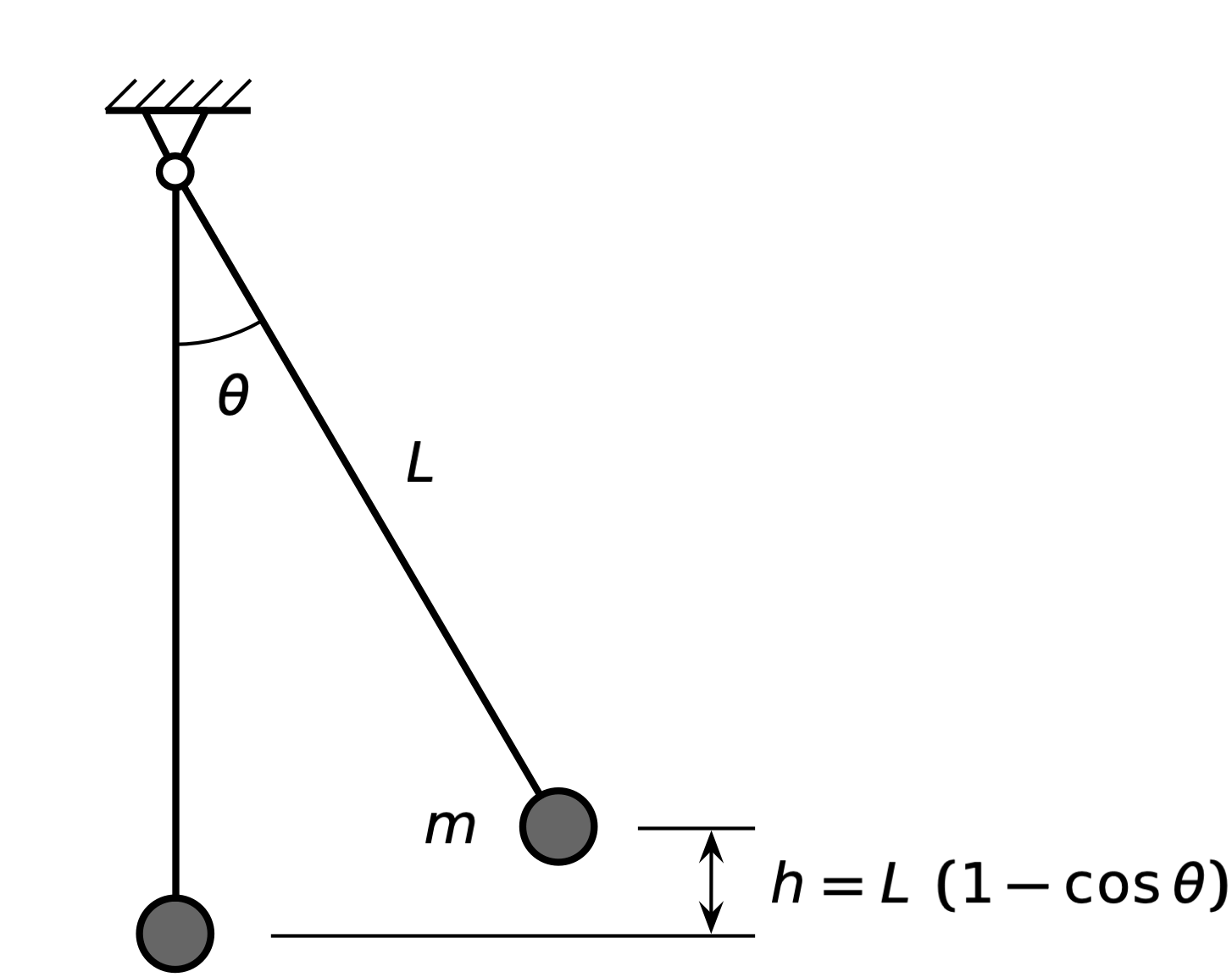
Getting back to the small angle approximation of cosine, the reason I knew to use it is it comes up so often in mechanics problems. Consider one of the most common mechanics problems, the oscillation of a pendulum:

Inspired by the French definition of the meter, we’ll use Lagrange’s Equation to derive the differential equation of the pendulum. For that, we need the kinetic and potential energies of the pendulum bob. The kinetic energy is easy:

$$T=\frac{1}{2}m{v}^2=\frac{1}{2}m{\left(L\dot{\theta }\right)}^2=\frac{1}{2}m{L}^2{\dot{\theta }}^2$$

where we’re using the overdot for the time derivative of $\theta$. That’s a notation due to Newton, so we can’t avoid the English entirely.

The potential energy is

$$U=mgh=mgL(1-\cos \theta )$$

And now you see how the Taylor series for cosine helps out for small angles. Using that, and dropping the approximately equals symbol, we get

$$U=\frac{1}{2}mgL{\theta }^2$$

This puts $T$ and $U$ into a very similar form. Plugging these into Lagrange’s equation,⁷

$$\frac{d}{dt}\left(\frac{\partial T}{\partial \dot{\theta }}\right)+\frac{\partial U}{\partial \theta }=0$$

leads to the familiar linear differential equation

$$\ddot{\theta }+\left(\frac{g}{L}\right)\theta =0$$

You can, of course use the exact expression for potential energy, derive the nonlinear differential equation,

$$\ddot{\theta }+\left(\frac{g}{L}\right)\sin \theta =0$$

and then linearize it by recognizing that $\sin \theta \approx \theta$. But it’s good to get in the habit of doing the small-angle approximations when working out the expressions for kinetic and potential energy. When you start dealing with multi-degree-of-freedom systems, you’ll find there are advantages to expressing the energies as quadratic forms:

$$T=\frac{1}{2}{\sum }_i{\sum }_j{A}_{ij}{\dot{x}}_i{\dot{x}}_{j}U=\frac{1}{2}{\sum }_i{\sum }_j{B}_{ij}{x}_i{x}_j$$

Or, in matrix form:

$$T=\frac{1}{2}{\dot{\mathbf{x}}}^T𝐀\dot{\mathbf{x}}U=\frac{1}{2}{𝐱}^T𝐁𝐱$$

It makes taking the partial derivatives much easier.

You might be wondering if there’s a more geometric way of showing that

$$h=\frac{1}{2}L{\theta }^2$$

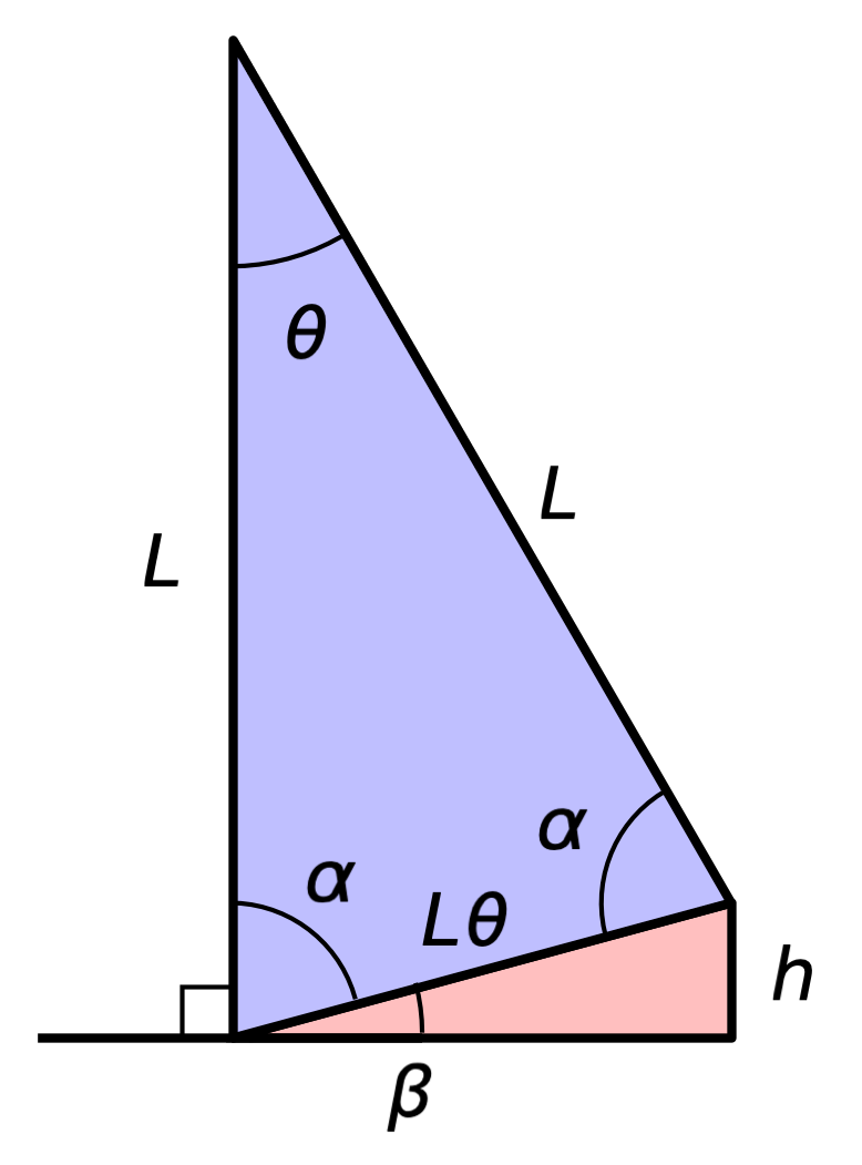
for small angles. Of course there is. Starting with the pendulum diagram shown above, form a (blue) triangle by connecting the pivot point and the two bob positions shown. They form another (pink) triangle whose height is $h$.

We know the blue triangle is isosceles because the two long legs are equal to the length of the pendulum, $L$. That means the two angles at the base are equal, and the rule for the sum of angles in a triangle tells us

$$2\alpha +\theta ={180}^{\circ }$$

or

$$\alpha +\frac{\theta }{2}={90}^{\circ }$$

The right angle between the vertical leg of the blue triangle and the horizontal leg of the pink triangle tells us

$$\alpha +\beta ={90}^{\circ }$$

and therefore

$$\beta =\frac{\theta }{2}$$

So far, we haven’t used any small-angle properties. Now we will. The hypotenuse of the pink triangle is the base of the blue triangle, and for small angle $\theta$, the length is $L\theta$. Therefore, the height of the pink triangle, $h$, is

$$h=\left(L\theta \right)\beta =\left(L\theta \right)\left(\frac{\theta }{2}\right)=\frac{1}{2}L{\theta }^2$$

So you can get the potential energy of the pendulum in a quadratic form even if you don’t know the Taylor series for cosine. Small angle theory is fun!

Getting back to the video, Matt shows that while polynomial approximations of some functions are nice and well-behaved, polynomial approximations of other functions can be terribly inaccurate, especially near the ends of the sample point interval. This, finally, is the Runge phenomenon.⁸

I knew about the Runge phenomenon before seeing Matt’s video, but I confess if you woke me from a deep sleep and asked me to describe it, my description would likely be of the Gibb’s phenomenon, which is similar.

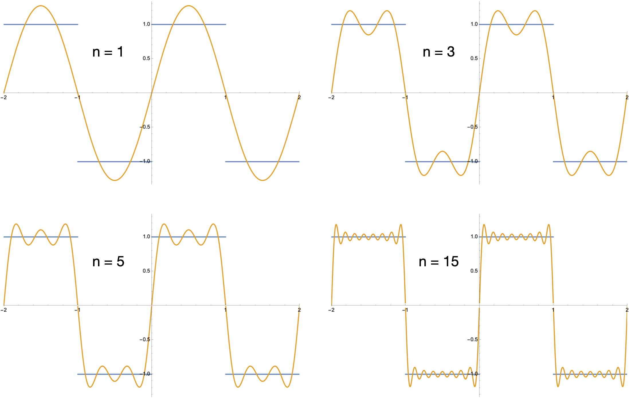
The classic example of the Gibbs phenomenon is the Fourier series expansion of a square wave. I’ve chosen the square wave to be antisymmetric with an amplitude of 1 and a period of 2. For this the Fourier series is

$${\sum }_{k=1,3,5,\dots }^n\frac{4}{k\pi }\sin (k\pi x)$$

and we can see the Gibbs phenomenon by plotting a few values of $n$:

The swings aren’t as wild as those Matt shows for the Runge phenomenon, but they’re present across all values of $x$.

In the video, Matt shows how you can avoid the Runge phenomenon by choosing sampling points that are not equally spaced. The spacing that smooths the error out comes from the zeros of the Chebyshev polynomials of the first kind, which are also the x-coordinates of points spread evenly around a semicircle. My favorite thing about Chebyshev polynomials of the first kind is that they’re usually given the symbol $T$, which seems weird until you realize that the transliteration of Chebyshev’s name from the Russian has itself taken some pretty wild swings. I’ve seen both Tchebychev and Tchebycheff in older books, which makes the $T$ seem more reasonable.

Maybe staying on a single topic isn’t as easy as I thought.

Next post Previous post

Site search

Meta

• drdrang at leancrew
• Blog archive
• RSS feed
• JSON feed
• Mastodon
• GitHub repositories

Recent posts

Credits

This work is licensed under a Creative Commons Attribution-Share Alike 3.0 Unported License.

© 2005–2023, Dr. Drang