Plenty of polygons
June 28, 2024 at 1:48 PM by Dr. Drang
John D. Cook wrote a fun geometry post yesterday, and I wanted to use Mathematica to generate my own versions of his images.
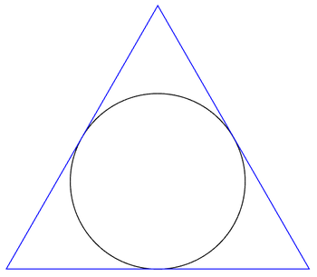
Start with a circle of unit radius and draw an equilateral triangle with sides that are tangent to the circle.

It wouldn’t take much to turn this into the Sign of the Deathly Hallows, but we have other things to do.
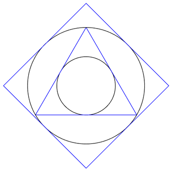
Draw a circle that passes through the vertices of the triangle and a square whose sides are tangent to the second circle.

Note that we drew the square with a corner at the 12:00 position. We’ll do that with all the polygons.
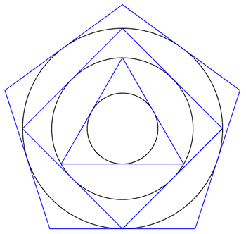
Continue by drawing a circle that passes through the corners of the square and a pentagon whose sides are tangent to that circle.

The radii of the circles have the following relationship to one another:
where is the radius of the circle that passes through the vertices of the n-sided polygon.
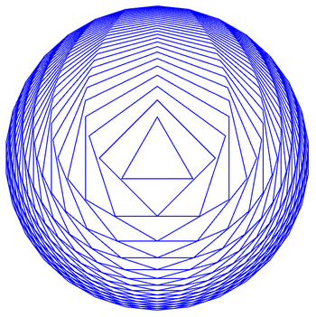
If we redo this drawing without showing the circles and continue adding sides to the circumscribing polygons (up to 30), we get this,

which is pretty cute.
Normally I wouldn’t repeat as much of someone else’s post, but I wanted to replicate all of Cook’s drawings myself in Mathematica.1 The images above were generated using this code:
The list of radii, saved in the variable r, is generated using the RecurrenceTable function in a straightforward translation of the formula above. The only thing you might be wondering about is why I added a term of zero to the front of the list. It’s because I wanted the indices of the r list to match the subscript in the formula.
The radii stored in r work perfectly as arguments to the RegularPolygon function. In Mathematica, the “radius” of a polygon is the radius of the circle that passes through the vertices, which matches our definition above. The only unusual thing needed in the calls to RegularPolygon is an angle argument of Pi/2 to orient the polygons with a vertex at the 12:00 position.
That pretty much does it for the geometry. The rest of the code consists of:
- Tweaks to the drawing commands to set colors, line thicknesses, and opacity.
- Export commands to create the PNG files you see above.
I’m still getting myself comfortable in Mathematica. Fun problems like this are a good way to extend myself.
-
I don’t know what Cook used for his drawings. He usually does his graphics in Python and Matplotlib, but he sometimes uses Mathematica. ↩
