Cauchy coup

July 19, 2025 at 10:03 PM by Dr. Drang

Bruce Ediger, who blogs at Information Camouflage, has been doing some interesting numerical experimentation recently; first in a post about estimating population size from a sample of serial numbers (you may have seen this Numberphile video on the same topic), and then a couple of videos about the Cauchy distribution. In the first, he looked at the sum of two random variables that are Cauchy distributed; in the second, he looked at the quotient of two normally distributed random variables, which—under certain conditions—is supposed to have a Cauchy distribution.

By numerical experimentation, I mean that Ediger’s generating sets of random numbers, doing some calculations on them, and then seeing how close his calculations are to certain theoretical results. It’s a good way to get a feel for how things work, and it’s the kind of analysis that’s really only possible because of the computational power we all have at our fingertips. This sort of playing around with thousands and thousands of numbers just wasn’t feasible when I was learning probability and statistics, and I’m jealous of today’s students.

What attacted my interest in Ediger’s post on the quotient of two normals was the possibility that I could do the problem analytically without too much effort—mainly because the same computational power that lets him mess around with a hundred thousand quotients of random samples also lets me do calculus and algebra without dropping terms or making other silly errors.

Cauchy from the quotient of two zero-mean normals

I started by making sure I could prove that the quotient of two zero-mean normals has a Cauchy distribution. The analysis in this section follows the structure outlined in Papoulis’s Probability, Random Variables, and Stochastic Processes.

We begin by looking at the general problem of the quotient of two random variables of any distribution. We’ll call the two random variables X and Y and their joint probability density function $f_{X Y} (x, y)$ .¹

We’ll call our quotient Z and define it this way:

Z = \frac{X}{Y}

To figure out the probability density function of Z, we’ll first look at its cumulative distribution function, $F_{Z} (z)$ , which is defined as the probability that $Z \leq z$ ,

F_{Z} (z) = P (Z \leq z)

This probability will be the volume under the joint PDF of X and Y over the region where $X / Y \leq z$ . That’ll be this integral:

F_{Z} (z) = \iint_{x / y \leq z} f_{X Y} (x, y) d x d y

And the domain over which we take the integral will be the blue region in this graph,

Quotient integration domain

where the region extends as far as $f_{X Y} (x, y)$ extends in the upper left and lower right directions.

If this doesn’t seem obvious to you, don’t worry, it isn’t. But think of it this way:

If $y > 0$ , then $x / y$ will be less than $z$ when $x$ is to the left of the $x = z y$ line.
If $y < 0$ , then $x / y$ will be less than $z$ when $x$ is to the right of the $x = z y$ line. Making $y$ negative flips the direction of the less-than sign.

With the integration domain defined, we can write the expression for $F_{Z} (z)$ like this:

F_{Z} (z) = \int_{0}^{\infty} \int_{- \infty}^{z y} f_{X Y} (x, y) d x d y + \int_{- \infty}^{0} \int_{z y}^{\infty} f_{X Y} (x, y) d x d y

To get the PDF of Z, we need to differentiate $F_{Z} (z)$ with respect to z. This is done through the Leibniz rule. Normally that would leave us with six terms, three for each of the two integrals above. But luckily for us, four of those terms are zero, leaving

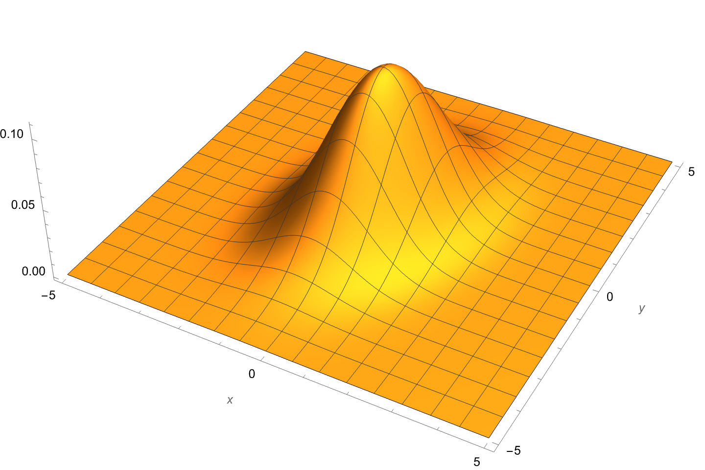
f_{Z} (z) = \int_{0}^{\infty} y f_{X Y} (z y, y) d y - \int_{- \infty}^{0} y f_{X Y} (z y, y) d y

Now it’s time to consider the case when X and Y are jointly normal. And to get to a Cauchy distribution for Z, both X and Y will have to have zero means. With that restriction, the joint density function will look something like this:

Joint normal surface plot

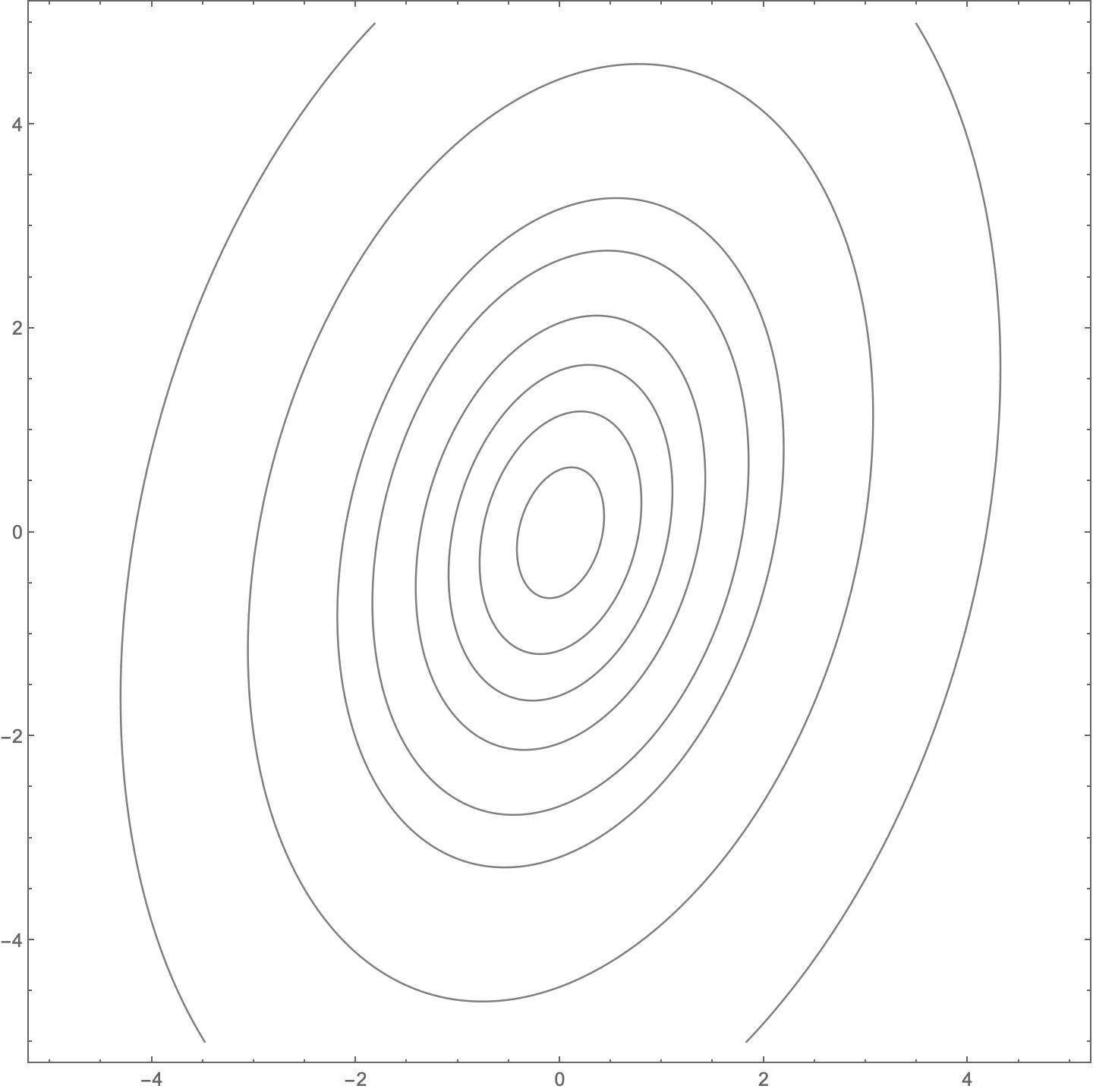
To make the plot, I needed some actual numbers, so I’ve given X a standard deviation of 1, Y a standard deviation of 1.5, and the correlation coefficient a value of 0.25. The analysis doesn’t rely on these or any other particular values for the parameters.

We can see the joint PDF’s structure a little better with a contour plot:

Joint normal contour plot

The key is that it has this kind of symmetry,

f_{X Y} (x, y) = f_{X Y} (- x, - y)

and we can take advantage of that symmetry to simplify the expression for $f_{Z} (z)$ :

f_{Z} (z) = 2 \int_{0}^{\infty} y f_{X Y} (z y, y) d y

OK, now we have to get into the nitty gritty and actually do some integration. Which means it’s time to abandon “by hand” analysis and switch to Mathematica. Here’s the notebook that does the following:

The integration to determine the form of $f_{Z} (z)$ . When writing stuff like this by hand, I would typically use $σ_{X}$ , $σ_{Y}$ , and $ρ$ for the standard deviations of X and Y and their correlation coefficient, but to make the typing easier in Mathematica, I use sx, sy, and r.
Checks the result against Papoulis’s. It’s not uncommon for Mathematica to give answers that don’t look like what you’ll find in a book, even though they are algebraically equivalent.
Determines the shape and location factors, $γ$ and $z_{0}$ , that put the result into the generic form for a Cauchy distribution that we see in the Wikipedia article:
$f_{Z} (z) = \frac{γ}{π [(z - z_{0})^{2} + γ^{2}]}$

Here’s the notebook:

So yes, the quotient of two zero-mean normals has a Cauchy distribution with a shape parameter of

γ = \frac{\sqrt{1 - ρ^{2}} σ_{X}}{σ_{Y}}

and a location parameter of

z_{0} = \frac{ρ σ_{X}}{σ_{Y}}

Ediger’s problem

That was sort of a warmup to make sure I understood how to use the MultinormalDistribution function. It’s time to move on to Ediger’s problem.

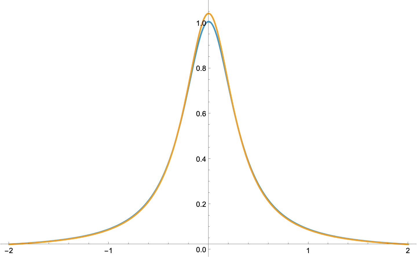
Ediger doesn’t take the quotient of two zero-mean normals. Instead, he takes the quotient of two independent ( $ρ = 0$ ) normals, one with zero mean and unit standard deviation, and the other with a mean of 1 and standard deviation of 3. This shouldn’t result in a Cauchy distribution, and it doesn’t. But to see how close it is, I made this Mathematica notebook:

Comparing the actual distribution of the quotient (in blue) with Ediger’s best fit of a Cauchy distribution (orange), we see this:

Exact PDF vs Ediger fit

Definitely not the same but pretty damned close.

Finally

I’m not sure most people would consider this recreational mathematics, but it’s recreational to me. You should see the things in my notebooks that don’t get turned into blog posts.

A habit I picked up from my thesis advisor is to use capital letters for random variables and their lower case versions for particular instances of those random variables. ↩

And now it’s all this

I just said what I said and it was wrong
Or was taken wrong

Cauchy coup

Cauchy from the quotient of two zero-mean normals

Ediger’s problem

Finally

Site search

Meta

Recent posts

Credits

And now it’s all this

I just said what I said and it was wrong Or was taken wrong

Cauchy coup

Cauchy from the quotient of two zero-mean normals

Ediger’s problem

Finally

Site search

Meta

Recent posts

Credits

I just said what I said and it was wrong
Or was taken wrong