Sparking joy
September 28, 2025 at 3:55 PM by Dr. Drang
I watched this Numberphile video a few days ago and learned not only about Harshad numbers, which I’d never heard of before, but also some new things about defining functions in Mathematica.
Harshad numbers1 are defined as integers that are divisible by the sum of their digits. For example,
so 42 is a Harshad number. On the other hand,
so 76 is not. You can use any base to determine whether a number is Harshad or not, but I’m going to stick to base 10 here.
After watching the video, I started playing around with Harshad numbers in Mathematica. Because Mathematica has both a DigitSum function and a Divisible function, it’s fairly easy to define a Boolean function that determines whether a number is Harshad or not:
myHarshadQ[n_] := Divisible[n, DigitSum[n]]
Mathematica functions that return Boolean values often end with Q (Divisible being an obvious exception), so that’s why I put a Q at the end of myHarshadQ. A couple of things to note:
- Both
DivisibleandDigitSumaccept and return lists. Therefore, we can givemyHarshadQa list of numbers and it will return a list of Boolean values. - Because
DigitSumaccepts only integer arguments,myHarshadQthrows an error if you feed it noninteger arguments.
To get all the Harshad numbers up through 100, we can use the Select and Range functions like this:
Select[Range[100], myHarshadQ]
which returns the list
{1, 2, 3, 4, 5, 6, 7, 8, 9, 10, 12,
 18, 20, 21, 24, 27, 30, 36, 40, 42, 45, 48,
 50, 54, 60, 63, 70, 72, 80, 81, 84, 90, 100}
You can check this against Sequence A005349 in the On-Line Encyclopedia of Integer Sequences.
There are a couple of ways to count how many Harshad numbers are in a given range. Either
Length[Select[Range[100], myHarshadQ]]
which is a straightforward extension of what we did above, or the less obvious
Count[myHarshadQ[Range[100]], True]
which works by making a list of 100 Boolean values and counting how many are True. The Count function is like Length, but it returns only the number of elements in a list that match a pattern. Both methods return the correct answer of 33, and they take about the same amount of time (as determined through the Timing function) to run.
While Mathematica doesn’t have a built-in function for determining whether a number is Harshad, it does have an external function, HarshadNumberQ, that does. This can be used in conjunction with ResourceFunction. The call
ResourceFunction["HarshadNumberQ"][42]
returns True. Similarly,
Select[Range[100], ResourceFunction["HarshadNumberQ"]]
returns the list of 33 numbers given above.
The resource function is considerably faster than mine. Running
Timing[Count[ResourceFunction["HarshadNumberQ"][Range[10000]], True]]
returns {0.027855, 1538}, while running
Timing[Count[myHarshadQ[Range[10000]], True]]
returns {0.06739, 1538}. The runtime, which is the first item in the list, changes slightly from one trial to the next, but myHarshadQ always takes nearly three times as long.
To figure out why, I downloaded the source notebook for HarshadNumberQ and took a look. Here’s the source code for the function:
SetAttributes[HarshadNumberQ, Listable];
iHarshadNumberQ[n_, b_] := Divisible[n, Total[IntegerDigits[n, Abs[b]]]]
HarshadNumberQ[n_Integer, b_Integer] :=
  With[{res = iHarshadNumberQ[Abs[n], b]}, res /; BooleanQ[res]]
HarshadNumberQ[n_Integer] := HarshadNumberQ[n, 10];
HarshadNumberQ[_, Repeated[_, {0, 1}]] := False
I won’t pretend to understand everything that’s going on here, but I have figured out a few things:
First, HarshadNumberQ is obviously defined to handle any number base, not just base-10. And it can handle a list of bases, too, so if you want to check on how many bases in which a number is Harshad, this is the function you want.
Second, HarshadNumberQ uses an argument pattern I’ve never seen before: n_Integer. This restricts it to accepting only integer inputs. It returns False when given noninteger arguments; it doesn’t just throw an error the way myHarshadQ does.
Third, HarshadNumberQ uses Total[IntegerDigits[n]] instead of DigitSum[n]. This, I believe, is at least part of the reason it runs faster than myHarshadQ. For example,
Timing[Total[IntegerDigits[99999^10]]]
returns {0.000084, 216}, while
Timing[DigitSum[99999^10]]
returns {0.000146, 216}.
Finally, the SetAttributes function is needed because Total would otherwise have trouble handling the output of IntegerDigits when the first argument is a list. Let’s look at some examples:
IntegerDigits[123456]
returns {1, 2, 3, 4, 5, 6}, a simple list that Total knows how to sum to 21. But
IntegerDigits[{12, 345, 6789}]
returns a lists of lists, {{1, 2}, {3, 4, 5}, {6, 7, 8, 9}}, which Total has trouble with. Calling
Total[IntegerDigits[{12, 345, 6789}]]
returns an error, saying that lists of unequal length cannot be added. We can get around this error by giving Total a second argument. Calling it as
Total[IntegerDigits[{12, 345, 6789}], {2}]
tells Total to add the second-level lists, returning {3, 12, 30}, which is just what we want. The problem is that this second argument to leads to an error when the first argument is a scalar instead of a list.
This, as best I can tell, is where the
SetAttributes[HarshadNumberQ, Listable];
line comes in. By telling Mathematica that HarshadNumberQ is Listable, we can define the function as if Total were always being used on scalars, and the system will thread over lists just like we want.
Since I’m just writing myHarshadQ for my own entertainment and not for others to use, I can take some of what I learned above and rewrite it to run faster. Like this:
SetAttributes[myHarshadQ, Listable];
myHarshadQ[n_] := Divisible[n, Total[IntegerDigits[n]]]
With this new definition, myHarshadQ runs considerably faster. Calling
Timing[Count[myHarshadQ[Range[10000]], True]]
returns {0.013527, 1538}. This is roughly twice as fast as HarshadNumberQ, probably because the definition doesn’t deal with other bases or handle errors gracefully.
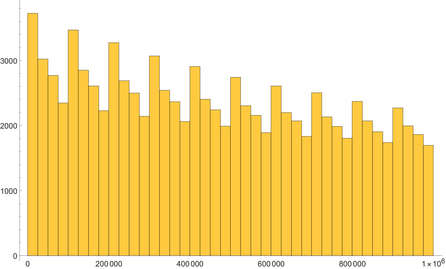
Now I can look at Harshad numbers over a broad range without having to wait long for results. To see how they’re distributed over the first million numbers, I ran
Histogram[Select[Range[999999], HarshadNumberQ], {25000}, ImageSize -> Large]
and got this histogram (with a bin width of 25,000):

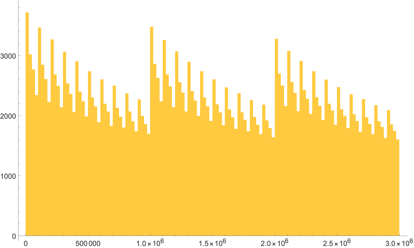
The stepdown pattern repeats every 100,000 numbers, moving down each time. Let’s stretch out the range to three million and see what happens.
Histogram[Select[Range[2999999], HarshadNumberQ], {25000}, ImageSize -> Large]

The pattern repeats at the larger scale, too.
If you want to learn some other Harshad facts, you should watch this extra footage at Numberphile. There doesn’t seem to be anything directly practical you can do with Harshad numbers, but you can use them to exercise your mathematical muscles. Or learn new things about the Wolfram Language.
-
You might think Harshad numbers are named after their discoverer or, in accordance with Stigler’s Law, their popularizer, but no. See either the video or the Wikipedia article for the origin of the name. ↩
