Semiautomated LaTeX tables
October 17, 2021 at 11:17 AM by Dr. Drang
As a followup to my last post about automating the creation of Markdown tables, here’s a simple pair of functions that’ve been very helpful in making LaTeX tables quickly.
A few years ago, I wrote about how much I hated the syntax of LaTeX tables and how I was shifting to building tables as graphics files that I could insert using the \includegraphics{} command. In the early stages, I was doing this by hand, as outlined in that post, but after I developed a sense of the kind of spacing I liked, I translated that into a set of Python functions that used the ReportLab module to create decent-looking tables as PDF files. A Python solution made the most sense, as the data from which I made the tables typically came out of data analysis done in Python.
The functions I wrote worked well enough, but the overall system was more fussy than it should have been, and I realized I’m better at programming the manipulation of text than the manipulation of graphics. So I started thinking about ways to make LaTeX tables directly from Python data.
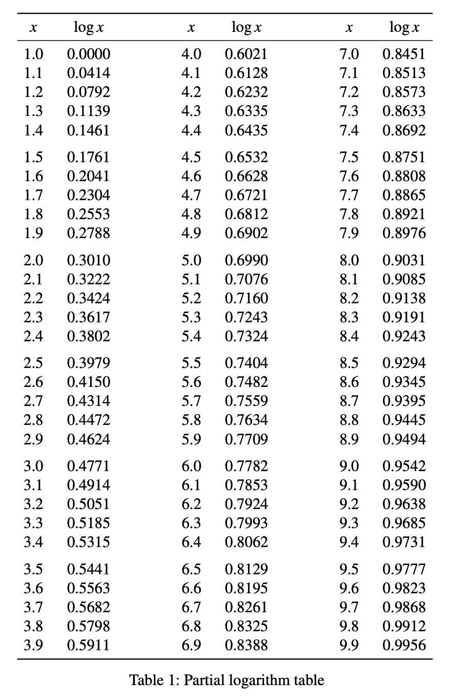
Here’s an artificial example that isn’t too far away from the kinds of tables I need to make. Let’s say we want a short table of (base 10) logarithms. We can generate the data—a list of values and a parallel list of their logs—like this:
python:
from math import log10

x = [ (10+i)/10 for i in range(90) ]
lx = [ f'{log10(y):.4f}' for y in x ]
And what I want is a table that looks like this:

I use the booktabs package for making tables. I like its clean look, and I like its nice \addlinespace command for adding a little extra space between certain rows to make reading long tables easier. The code that produced the table above is
\setlength{\tabcolsep}{.125in}
\begin{table}[htbp]
\begin{center}
\begin{tabular}{
    @{\hspace*{5pt}}
    cc@{\hspace{.75in}}cc@{\hspace{.75in}}cc
    @{\hspace*{5pt}}
}
\toprule
$x$ & $\log x$ & $x$ & $\log x$ & $x$ & $\log x$ \\
\midrule
1.0 & 0.0000 & 4.0 & 0.6021 & 7.0 & 0.8451 \\
1.1 & 0.0414 & 4.1 & 0.6128 & 7.1 & 0.8513 \\
1.2 & 0.0792 & 4.2 & 0.6232 & 7.2 & 0.8573 \\
1.3 & 0.1139 & 4.3 & 0.6335 & 7.3 & 0.8633 \\
1.4 & 0.1461 & 4.4 & 0.6435 & 7.4 & 0.8692 \\
\addlinespace
1.5 & 0.1761 & 4.5 & 0.6532 & 7.5 & 0.8751 \\
    .
    .
    .
3.7 & 0.5682 & 6.7 & 0.8261 & 9.7 & 0.9868 \\
3.8 & 0.5798 & 6.8 & 0.8325 & 9.8 & 0.9912 \\
3.9 & 0.5911 & 6.9 & 0.8388 & 9.9 & 0.9956 \\
\bottomrule
\end{tabular}
\caption{Partial logarithm table}
\label{table}
\end{center}
\end{table}
The boilerplate at the top and bottom is produced by a Keyboard Maestro macro. Except for the column alignment line and caption—which need to be set for each table—it never changes. The troublesome parts are the header and, especially, the body. For those, I use two functions, theader and tbody, to build the LaTeX code without having to touch the ampersand or backslash keys. To make the table in the same script as the data, I adjust the script to this:
python:
from math import log10
from latex_tables import tbody, theader

x = [ (10+i)/10 for i in range(90) ]
lx = [ f'{log10(y):.4f}' for y in x ]
headers = ['$x$', '$\log x$']*3
print(theader(headers))
print(tbody(x[:30], lx[:30], x[30:60], lx[30:60], x[60:], lx[60:], group=5))
The output is
$x$ & $\log x$ & $x$ & $\log x$ & $x$ & $\log x$ \\
\midrule
1.0 & 0.0000 & 4.0 & 0.6021 & 7.0 & 0.8451 \\
1.1 & 0.0414 & 4.1 & 0.6128 & 7.1 & 0.8513 \\
1.2 & 0.0792 & 4.2 & 0.6232 & 7.2 & 0.8573 \\
1.3 & 0.1139 & 4.3 & 0.6335 & 7.3 & 0.8633 \\
1.4 & 0.1461 & 4.4 & 0.6435 & 7.4 & 0.8692 \\
\addlinespace
1.5 & 0.1761 & 4.5 & 0.6532 & 7.5 & 0.8751 \\
    .
    .
    .
3.7 & 0.5682 & 6.7 & 0.8261 & 9.7 & 0.9868 \\
3.8 & 0.5798 & 6.8 & 0.8325 & 9.8 & 0.9912 \\
3.9 & 0.5911 & 6.9 & 0.8388 & 9.9 & 0.9956 \\
which, as you can see, is exactly what goes between the top and bottom boilerplate.
The functions are defined in the file latex_tables.py, which is saved in my site-packages directory. Here’s the code:
python:
 1:  def tbody(*cols, group=0):
 2:    "Given the columns, return the body of a LaTeX table."
 3:
 4:    # Add blanks at the ends of short columns
 5:    lens = [ len(c) for c in cols ]
 6:    nrows = max(lens)
 7:    cols = [ c + [' ']*(nrows - len(c)) for c in cols ]
 8:
 9:    # Assemble the rows of the table
10:    rows = []
11:    for i in range(nrows):
12:      if (group > 0) and (i > 0) and (i % group == 0):
13:        rows.append(r'\addlinespace')
14:      row = [ str(c[i]) for c in cols ]
15:      rows.append(' & '.join(row) + r' \\')
16:
17:    return '\n'.join(rows)
18:
19:  def theader(hcols):
20:    "Given a list of column headers, return the header lines of a LaTeX table."
21:
22:    # Figure out the maximum number of lines in the header
23:    hcols = [ x.splitlines() for x in hcols ]
24:    maxlines = max(len(x) for x in hcols)
25:    hcols = [ [' ']*(maxlines - len(x)) + x for x in hcols ]
26:
27:    # Assemble the rows of the header
28:    rows = []
29:    for i in range(maxlines):
30:      row = [ str(c[i]) for c in hcols ]
31:      rows.append(' & '.join(row) + r' \\')
32:
33:    return '\n'.join(rows) + '\n\\midrule'
Like the example log table, most of the tables I make come from lists of data that are meant to go into the columns of the table. So the main feature of tbody is assembling the rows from those lists. The other significant feature is placing the \addlinespace command according to the group parameter.
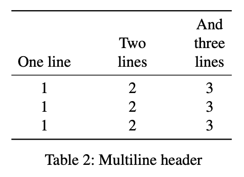
The theader function is even simpler. The only interesting thing about it is how it handles multiline headers. If it’s called like this,
print(theader(['One line', 'Two\nlines', 'And\nthree\nlines']))
the output will be
    &   & And \\
    & Two & three \\
One line & lines & lines \\
\midrule
which will produce a table that has a header that looks like this:

The header lines are bottom-aligned instead of top-aligned. The main purpose of theader is to automate that alignment.
Trickier table arrangements still have me hauling out my copy of Kopka & Daly, but theader and tbody do the bulk of the work even in those cases.
