And now it’s all this

I just said what I said and it was wrong
Or was taken wrong

Next post Previous post

Catenaries, parabolas, and ropes

March 20, 2022 at 3:00 PM by Dr. Drang

Picking up from the last post, let’s think about how and why a parabola could be a good approximations to a catenary.

To get a sense of where we’re going, let’s do some numerical experimentation. We’ll start with a catenary of about the same dimensions as last week’s, 40 units wide and 40 units high, but this time we’ll flip it back to the usual orientation, with the ends high and the center low. And we’ll adopt a more common terminology, in which the width, $w$, is called the span, and the height, $h$, is called the sag.

If we put the origin of our coordinate system at the center of catenary, the formula will be

$$y=a(\cosh \frac{x}{a}-1)$$

where $\cosh$ is the hyperbolic cosine. The parameter $a$ is the solution to the equation

$$a(\cosh \frac{w}{2a}-1)=h$$

which is

$$a=8.10867$$

for this span and sag.

A parabola that fits the catenary at the end points and the center has the formula

$$y=h{\left(\frac{2x}{w}\right)}^2$$

or

$$y=\frac{x^2}{10}$$

for this span and sag.

Here’s what they look like, with the catenary in orange and the parabola in blue:

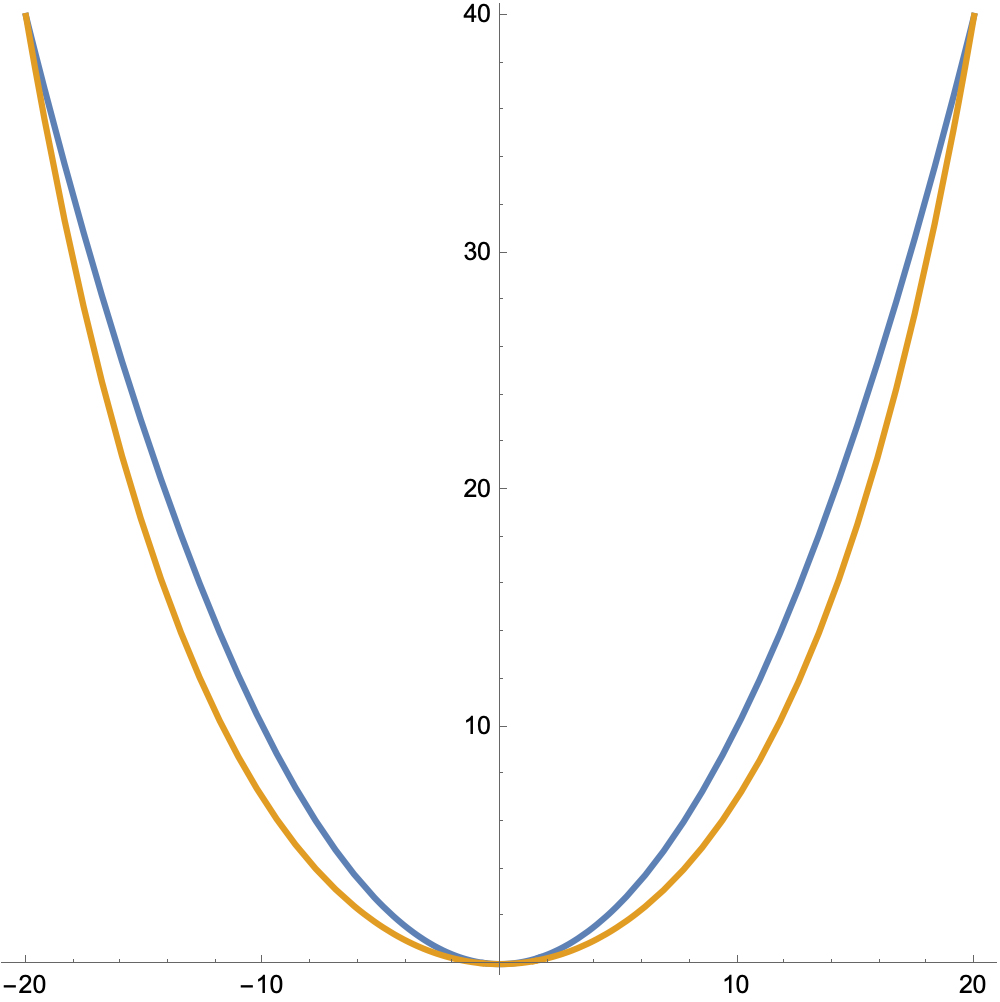
The parabola isn’t a particularly good fit. It’s maximum deviation from the catenary is 4.2 units, or about 10% of the sag. We could, of course, have gotten a better fit overall if we hadn’t forced the parabola to fit perfectly at the ends and the center. But no matter what fitting technique we used, no parabola would be a good match to a catenary with this high a sag/span ratio.

So let’s look at a catenary/parabola pair with half the sag. We’ll bypass the numbers and go straight to the plots:

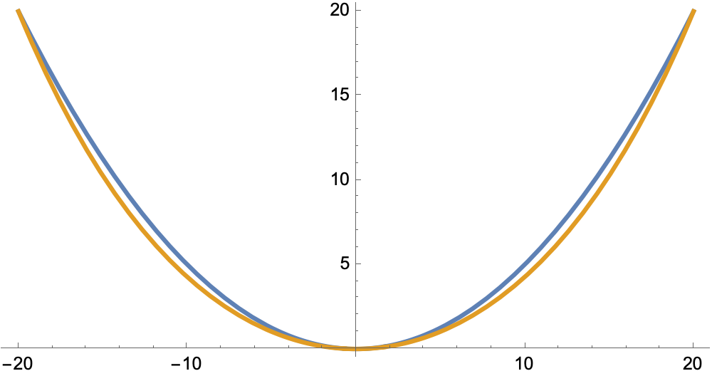
Looks better, doesn’t it? And not just on an absolute basis. The maximum deviation is now about 5% of the sag.

Cutting the sag in half once again, we get this:

Now the maximum deviation is less than 2% of the sag.

One more, this time with a sag one-eight of the span.

Now the two curves are basically indistinguishable. The maximum deviation is just under 0.5% of the sag.

These examples suggest the parabola makes for a pretty good estimate of a catenary if the sag is relatively small. We could go back to the equations and do a series expansion of the hyperbolic cosine—and we will do that later—but I find it more satisfying to look at the structural mechanics that leads to the equations in the first place.

---

We’ll start with a rope¹ subjected to tension, $T$, and a vertical load, $q$. Neither of these forces are necessarily constant.

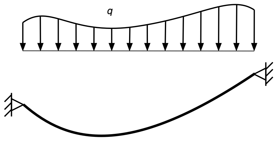
I’ve drawn the vertical load above the rope to avoid a messy drawing and to make it clear that it varies in the horizontal direction.

Here’s a free-body diagram of a differential segment of the rope:

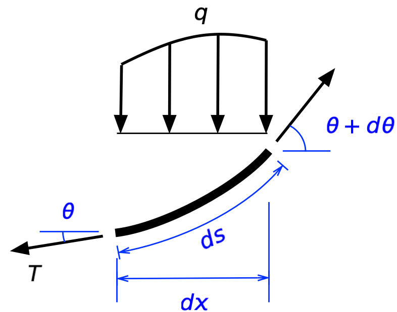
Horizontal equilibrium says

$$(T+dT)\cos (\theta +d\theta )-T\cos \theta =0$$

or

$$\frac{d(T\cos \theta )}{dx}=0$$

Since $T\cos \theta$ is the horizontal component of the tension in the rope, which we’ll call $H$, this says that $H$ is constant, which turns out to be a useful thing to know.

Vertical equilibrium is a bit trickier.

$$(T+dT)\sin (\theta +d\theta )-T\sin \theta -qdx=0$$ $$\frac{d(T\sin \theta )}{dx}=q$$

Since $H=T\cos \theta$, we can substitute in for $T$ to get

$$\frac{d\left(\frac{H}{\cos \theta }\sin \theta \right)}{dx}=H\frac{d(\tan \theta )}{dx}=q$$

By definition,

$$\tan \theta =\frac{dy}{dx}=y^{\prime }$$

so

$$\frac{d{y}^{\prime }}{dx}=\frac{d^{2}y}{d{x}^2}=y^{\prime \prime }=\frac{q}{H}$$

The solution to this differential equation depends of the form of $q$. Note that the way we’ve defined it, $q$ is the vertical force per unit of length in the horizontal direction, not per unit of length along the rope. So for the catenary problem, where the rope is taken to have constant weight along its length, $q$ is some function of the slope. To get that function, we apply the same ideas used to calculate arc length, where

$$ds=\sqrt{d{x}^2+d{y}^2}=dx\sqrt{1+(y^{\prime }{)}^2}$$

If the weight per unit length of the rope is $q_0$ (a constant), the weight of a differential segment of rope is

$$q_{0}ds=q_0\sqrt{1+(y^{\prime }{)}^2}dx$$

This means the weight per unit of horizontal length is

$$q=q_0\sqrt{1+(y^{\prime }{)}^2}$$

and our differential equation for the catenary becomes

$$y^{\prime \prime }=\frac{q_0}{H}\sqrt{1+(y^{\prime }{)}^2}$$

This is a solvable differential equation (we’ll get to its solution in a minute), but let’s first consider a simplification.

---

If the rope is held tight enough to keep the slope small over its entire length, $(y^{\prime }{)}^2$ will be small compared to $1$, and the equation will be reasonably approximated by

$$y^{\prime \prime }=\frac{q_0}{H}$$

In other words, if slope is small everywhere, the weight per unit length in the horizontal direction will be nearly uniform and equal to the weight per unit length along the rope.

With the second derivative equal to a constant, it should be clear that the solution to this simplified equation is a parabola,

$$y=\frac{1}{2}\frac{q_0}{H}{x}^2+C_{1}x+C_0$$

If we set up our coordinate system as above with the origin at the bottom of the sag, both $y$ and $y^{\prime }$ will be zero at $x=0$, and the constants of integration will fall out, leaving

$$y=\frac{1}{2}\frac{q_0}{H}{x}^2$$

To figure out how $q_0$ and $H$ are related to the sag and span, we can simply evaluate this equation at the right end of the rope, where $x=w/2$ and $y=h$:

$$h=\frac{1}{2}\frac{q_0}{H}{\left(\frac{w}{2}\right)}^2$$

We can rearrange this into a more useful nondimensional form:

$$\frac{h}{w}=\frac{1}{8}\left(\frac{q_{0}w}{H}\right)$$

Note that $q_{0}w$ is, approximately, the weight of the rope, so the term in the parentheses is the ratio of the total weight of the rope to the horizontal component of tension.

There’s another way to get this relationship. Consider a free-body diagram of the right half of the rope (where I’ve exaggerated the sag for clarity):

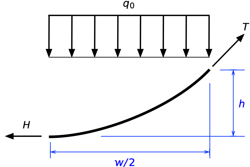
Because the slope at the bottom of the sag is zero, the tension in the rope there is $H$. Taking the moment about the upper right end gives us

$$q_0\left(\frac{w}{2}\right)\left(\frac{w}{4}\right)-Hh=0$$

or

$$\frac{h}{w}=\frac{1}{8}\left(\frac{q_{0}w}{H}\right)$$

as before. Structural engineers usually prefer this approach because it’s a more physical explanation of the relationship.

---

Now let’s return to the original differential equation,

$$y^{\prime \prime }=\frac{q_0}{H}\sqrt{1+(y^{\prime }{)}^2}$$

The solution—which you can get by a change of variable and then separation of variables (or by using software like SymPy or Mathematica)—is

$$y=\frac{H}{q_0}\cosh (\frac{q_{0}x}{H}+C_1)+C_0$$

As above, $y(0)=0$ and $y^{\prime }(0)=0$, so the constants of integration work out to

$$C_0=-\frac{H}{q_0},C_1=0$$

so

$$y=\frac{H}{q_0}[\cosh \left(\frac{q_{0}x}{H}\right)-1]$$

We figure out how $q_0$ and $H$ are related to the sag and span by evaluating this expression at the right end of the rope:

$$y\left(\frac{w}{2}\right)=h=\frac{H}{q_0}[\cosh \left(\frac{q_{0}w}{2H}\right)-1]$$

Dividing through by $w$ gives us a nondimensional expression,

$$\frac{h}{w}=\frac{H}{q_{0}w}[\cosh \left(\frac{1}{2}\frac{q_{0}w}{H}\right)-1]$$

This is not an expression with a simple algebraic solution. In general, we’ll have to solve it numerically, but we can see what the solution will be like for a small sag/span ratio by considering the Taylor series expansion of the hyperbolic cosine about zero:

$$\cosh u=1+\frac{u^2}{2}+\frac{u^4}{24}+\dots$$

Plugging this into the expression above gives

$$\frac{h}{w}=\frac{H}{q_{0}w}([1+\frac{1}{2}{\left(\frac{q_{0}w}{2H}\right)}^2+\frac{1}{24}{\left(\frac{q_{0}w}{2H}\right)}^4+\dots ]-1)$$

and therefore

$$\frac{h}{w}=\frac{1}{8}\left(\frac{q_{0}w}{H}\right)+\frac{1}{384}{\left(\frac{q_{0}w}{H}\right)}^3+\dots \approx \frac{1}{8}\left(\frac{q_{0}w}{H}\right)$$

This matches both our expectations from the simplification of the differential equation and our numerical experimentation at the beginning of the post. A shallow catenary is nearly a parabola because the weight per unit of horizontal length of a shallow catenary is nearly constant.

Although the example shown here has the ends of the rope at the same elevation, the differential equation works for any set of end points. The solution is always a catenary, and the catenary can be approximated by a parabola if the sag is relatively small.

---

Because the cables used in structural applications typically have little sag, the parabolic approximation can be very useful. I used it many years ago when investigating an accident involving a crane with a multi-prong hook that was lifting an offshore oil platform. Eight cables were strung between the hook and various lifting lugs built into the platform. Shortly after the platform got up in the air, one of the prongs of the hook snapped and the platform fell. Much damage to both the platform and the crane.

Because this lift was such a massive undertaking—the hook was designed to carry 5,000 tons, and the platform was somewhere in that neighborhood—there were lots of photos taken before, during, and after the accident. I was able to estimate the sag in each cable from the photos and then used those values to calculate all the cable tensions shortly before the hook broke. Although the idea behind the lift was to distribute the weight of the platform relatively equally, my calculations showed that most of the load was being carried by just a few of the cables. As Murphy’s Law would have it, two of the cables carrying the highest loads were slung over a prong that had a significant casting defect. The combination of a weak prong and higher-than-expected loads led to the failure.

Next post Previous post

Site search

Meta

• drdrang at leancrew
• Blog archive
• RSS feed
• JSON feed
• Mastodon
• GitHub repositories

Recent posts

Credits

This work is licensed under a Creative Commons Attribution-Share Alike 3.0 Unported License.

© 2005–2023, Dr. Drang