More general sunrise/sunset plots
November 11, 2023 at 11:47 AM by Dr. Drang
I recently did that thing we’ve all done, where I kept working on a problem, refining the solution far beyond its value. I don’t think it’s necessarily wrong to overwork a problem—I always learn from the experience, and the reason I keep at it is that I’m having fun making the little improvements. And sometimes I get a blog post out of it.
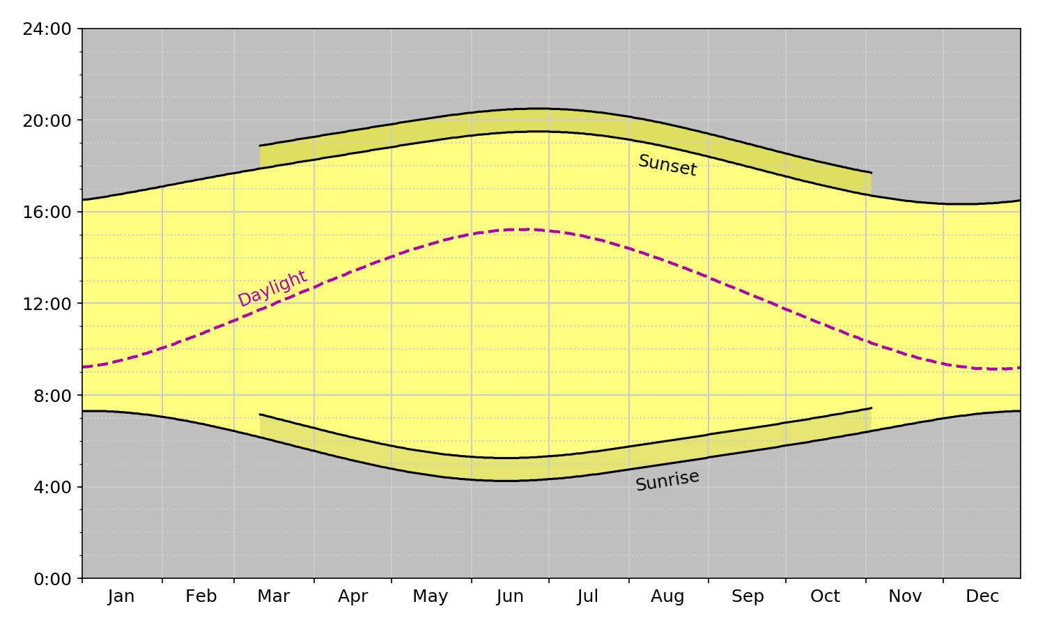
Earlier this week, Michael Glotzer on Mastodon reminded me of a little script I wrote about 5 years ago that made this sunrise/sunset plot for Chicago:

As I said at the time, there were several bespoke aspects to the script that built this plot. I did a lot of hand-editing of the US Naval Observatory data that was the script’s input. Also, the “Sunrise,” “Sunset,” and “Daylight” curve labels were set at positions and angles that were specific to the plot; they’d have to be redone if I wanted to make a plot for another city. To generalize the script to handle any set of USNO sunrise/sunset data, I’d have to alter the code to do the following:
- Read the data directly from the USNO text without editing.
- Add titles containing the location and year so the plots could be distinguished from one another.
- Change the way the curve labels were positioned to make them look good for any curve.
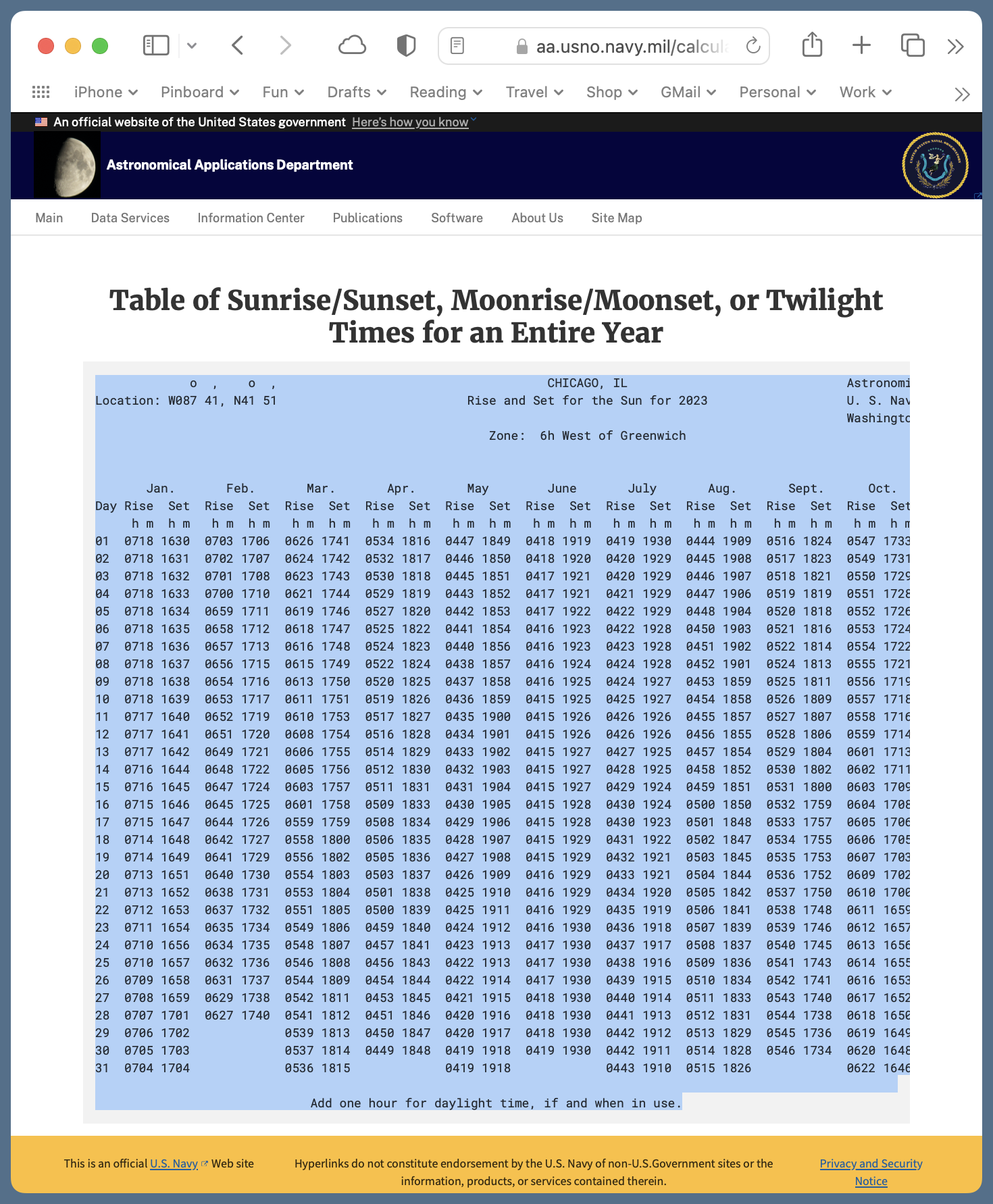
My goal was to feed the data to my script through standard input. I’d choose the location and year on the USNO site, copy the text that appears on the followup page,

and then pipe the text on the clipboard to my script via pbpaste:
pbpaste | sunplot
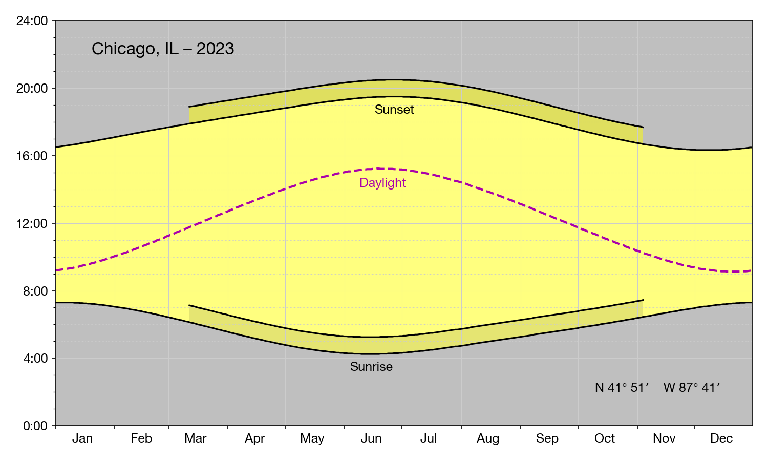
The result would be a PNG file in the current working directory, named according to the location and year—in this case, Chicago, IL-2023.png.

As you can see, I’ve added the name and year as a title in the upper left corner and the latitude and longitude in the lower right corner. Also, the curves are labeled at their peaks or valleys, as appropriate. As before, the main curves are given in Standard Time (as the USNO presents it in its tables) and the curves associated with the darker yellow are given in Daylight Saving Time.
Here’s the code for sunplot:
python:
  1:  #!/usr/bin/env python
  2:
  3:  import sys
  4:  import re
  5:  from dateutil.parser import parse
  6:  from datetime import datetime
  7:  from datetime import timedelta
  8:  from matplotlib import pyplot as plt
  9:  import matplotlib.dates as mdates
 10:  from matplotlib.ticker import MultipleLocator, FormatStrFormatter
 11:
 12:
 13:  # Functions
 14:
 15:  def headerInfo(header):
 16:    "Return location name, coordinates, and year from the USNO header lines."
 17:
 18:    # Get the place name from the middle of the top line
 19:    left = 'o  ,    o  ,'
 20:    right = 'Astronomical Applications Dept.'
 21:    placeName = re.search(rf'{left}(.+){right}', header[0]).group(1).strip()
 22:
 23:    # If the place name ends with a comma, a space, and a pair of capitals,
 24:    # assume it's in location, ST format and capitalize the location while
 25:    # keeping the state as all uppercase. Otherwise, capitalize all the words.
 26:    if re.match(r', [A-Z][A-Z]', placeName[-4:]):
 27:      placeParts = placeName.split(', ')
 28:      location = ', '.join(placeParts[:-1]).title()
 29:      state = placeParts[-1]
 30:      placeName = f'{location}, {state}'
 31:    else:
 32:      placeName = placeName.title()
 33:
 34:    # The year is at a specific spot on the second line
 35:    year = int(header[1][80:84])
 36:
 37:    # The latitude and longitude are at specific spots on the second line
 38:    longString = header[1][10:17]
 39:    latString = header[1][19:25]
 40:
 41:    # Reformat the latitude into d° m′ N format (could be S)
 42:    dir = latString[0]
 43:    degree, minute = latString[1:].split()
 44:    lat = f'{int(degree)}° {int(minute)}′ {dir}'
 45:
 46:    # Reformat the longitude into d° m′ W format
 47:    dir = longString[0]
 48:    degree, minute = longString[1:].split()
 49:    long = f'{int(degree)}° {int(minute)}′ {dir}'
 50:
 51:    return placeName, lat, long, year
 52:
 53:  def bodyInfo(body, isLeap):
 54:    "Return lists of sunrise, sunset, and daylight length hours from the USNO body lines."
 55:
 56:    # Initialize
 57:    sunrises = []
 58:    sunsets = []
 59:    lengths = []
 60:
 61:    # Lengths of monthly columns
 62:    if isLeap:
 63:      daysInMonth = [31, 29, 31, 30, 31, 30, 31, 31, 30, 31, 30, 31]
 64:    else:
 65:      daysInMonth = [31, 28, 31, 30, 31, 30, 31, 31, 30, 31, 30, 31]
 66:
 67:    # Rise and set character start positions for each month
 68:    risePos = [ 4 + 11*i for i in range(12) ]
 69:    setPos = [ 9 + 11*i for i in range(12) ]
 70:
 71:    # Collect data from each day
 72:    for m in range(12):
 73:      for d in range(daysInMonth[m]):
 74:        riseString = body[d][risePos[m]:risePos[m]+4]
 75:        hour, minute = int(riseString[:2]), int(riseString[-2:])
 76:        sunrise = hour + minute/60
 77:        setString = body[d][setPos[m]:setPos[m]+4]
 78:        hour, minute = int(setString[:2]), int(setString[-2:])
 79:        sunset = hour + minute/60
 80:        sunrises.append(sunrise)
 81:        sunsets.append(sunset)
 82:        lengths.append(sunset - sunrise)
 83:
 84:    return(sunrises, sunsets, lengths)
 85:
 86:  def dstBounds(year):
 87:    "Return the DST start and end day indices according to current US rules."
 88:
 89:    # Start DST on second Sunday of March
 90:    d = 8
 91:    while datetime.weekday(dstStart := datetime(year, 3, d)) != 6:
 92:      d += 1
 93:    dstStart = (dstStart - datetime(year, 1, 1)).days
 94:
 95:    # End DST on first Sunday of November
 96:    d = 1
 97:    while datetime.weekday(dstEnd := datetime(year, 11, d)) != 6:
 98:      d += 1
 99:    dstEnd = (dstEnd - datetime(year, 1, 1)).days
100:
101:    return dstStart, dstEnd
102:
103:  def centerPeak(data):
104:    "Return the maximum value and the index of its central position."
105:
106:    peak = max(data)
107:    # Average (to the nearest integer) the first and last peak indices
108:    peakPos = (data.index(peak) + (len(data) - data[-1::-1].index(peak))) // 2
109:    return peak, peakPos
110:
111:  def centerValley(data):
112:    "Return the minimum value and the index of its central position."
113:
114:    valley = min(data)
115:    # Average (to the nearest integer) the first and last valley indices
116:    valleyPos = (data.index(valley) + (len(data) - data[-1::-1].index(valley))) // 2
117:    return valley, valleyPos
118:
119:
120:  # Start processing
121:
122:  # Read the USNO data from stdin into a list of lines.
123:  # Text should come from https://aa.usno.navy.mil/data/RS_OneYear
124:  usno = sys.stdin.readlines()
125:
126:  # Get location and year from header
127:  placeName, lat, long, year = headerInfo(usno[:2])
128:
129:  # Is it a leap year?
130:  isLeap = (year % 400 == 0) or ((year % 4 == 0) and not (year % 100 == 0))
131:
132:  # Get sunrise, sunset, and sunlight length lists from body
133:  sunrises, sunsets, lengths = bodyInfo(usno[9:], isLeap)
134:
135:  # Generate list of days for the year
136:  currentDay = datetime(year, 1, 1)
137:  lastDay = datetime(year, 12, 31)
138:  days = [currentDay]
139:  while (currentDay := currentDay + timedelta(days=1)) <= lastDay:
140:    days.append(currentDay)
141:
142:  # The portion of the year that uses DST
143:  dstStart, dstEnd = dstBounds(year)
144:  dstDays = days[dstStart:dstEnd]
145:  dstRises = [ x + 1 for x in sunrises[dstStart:dstEnd] ]
146:  dstSets = [ x + 1 for x in sunsets[dstStart:dstEnd] ]
147:
148:  # Plot the data
149:  fig, ax =plt.subplots(figsize=(10,6))
150:
151:  # Shaded areas
152:  plt.fill_between(days, sunrises, sunsets, facecolor='yellow', alpha=.5)
153:  plt.fill_between(days, 0, sunrises, facecolor='black', alpha=.25)
154:  plt.fill_between(days, sunsets, 24, facecolor='black', alpha=.25)
155:  plt.fill_between(dstDays, sunsets[dstStart:dstEnd], dstSets, facecolor='yellow', alpha=.5)
156:  plt.fill_between(dstDays, sunrises[dstStart:dstEnd], dstRises, facecolor='black', alpha=.1)
157:
158:  # Curves
159:  plt.plot(days, sunrises, color='k')
160:  plt.plot(days, sunsets, color='k')
161:  plt.plot(dstDays, dstRises, color='k')
162:  plt.plot(dstDays, dstSets, color='k')
163:  plt.plot(days, lengths, color='#aa00aa', linestyle='--', lw=2)
164:
165:  # Curve annotations centered on the peaks and valleys
166:  # To get these labels near the middle of the plot, we need to use
167:  # different functions for the northern and southern hemispheres
168:  riseFcn = {'N':centerValley, 'S':centerPeak}
169:  setFcn = {'N':centerPeak, 'S':centerValley}
170:  lengthFcn = {'N':centerPeak, 'S':centerValley}
171:
172:  # Sunrise
173:  labeledRise, labeledRiseIndex = riseFcn[lat[-1]](sunrises)
174:  ax.text(days[labeledRiseIndex], labeledRise - 1, 'Sunrise', fontsize=12, color='black', ha='center')
175:
176:  # Sunset
177:  labeledSet, labeledSetIndex = setFcn[lat[-1]](sunsets)
178:  ax.text(days[labeledSetIndex], labeledSet - 1, 'Sunset', fontsize=12, color='black', ha='center')
179:
180:  # Daylight length
181:  labeledLight, labeledLightIndex = lengthFcn[lat[-1]](lengths)
182:  ax.text(days[labeledLightIndex], labeledLight + .75, 'Daylight', fontsize=12, color='#aa00aa', ha='center')
183:
184:  # Place name and year in upper left; coordinates in lower right
185:  ax.text(datetime(year, 1, 20), 22, f'{placeName} – {year}', fontsize=16, color='black', ha='left')
186:  ax.text(datetime(year, 10, 10), 2, f'{lat},  {long}', fontsize=12, color='black', ha='left')
187:
188:  # Background grids
189:  ax.grid(which='major', color='#cccccc', ls='-', lw=.5)
190:  ax.grid(which='minor', color='#cccccc', ls=':', lw=.5)
191:
192:  # Horizontal axis shows month abbreviations between ticks
193:  ax.tick_params(axis='both', which='major', labelsize=12)
194:  plt.xlim(datetime(year, 1, 1), datetime(year, 12, 31))
195:  m = mdates.MonthLocator(bymonthday=1)
196:  mfmt = mdates.DateFormatter('               %b')
197:  ax.xaxis.set_major_locator(m)
198:  ax.xaxis.set_major_formatter(mfmt)
199:
200:  # Vertical axis labels formatted like h:mm
201:  plt.ylim(0, 24)
202:  ymajor = MultipleLocator(4)
203:  yminor = MultipleLocator(1)
204:  tfmt = FormatStrFormatter('%d:00')
205:  ax.yaxis.set_major_locator(ymajor)
206:  ax.yaxis.set_minor_locator(yminor)
207:  ax.yaxis.set_major_formatter(tfmt)
208:
209:  # Tighten up the white border and save
210:  fig.set_tight_layout({'pad': 1.5})
211:  plt.savefig(f'{placeName}-{year}.png', format='png', dpi=150)
For me, a 200-line script is pretty long. A lot of that is due to the continual tweaking I did to make it more general, more accommodating of different inputs.
The sunrise and sunset data is read in from standard input on Line 122 and stored in a list of lines. Here’s an example:
             o  ,    o  ,                                     CHICAGO, IL                              Astronomical Applications Dept.
Location: W087 41, N41 51                          Rise and Set for the Sun for 2023                   U. S. Naval Observatory
                                                                                                       Washington, DC  20392-5420
                                                      Zone:  6h West of Greenwich


       Jan.       Feb.       Mar.       Apr.       May        June       July       Aug.       Sept.      Oct.       Nov.       Dec.
Day Rise  Set  Rise  Set  Rise  Set  Rise  Set  Rise  Set  Rise  Set  Rise  Set  Rise  Set  Rise  Set  Rise  Set  Rise  Set  Rise  Set
     h m  h m   h m  h m   h m  h m   h m  h m   h m  h m   h m  h m   h m  h m   h m  h m   h m  h m   h m  h m   h m  h m   h m  h m
01  0718 1630  0703 1706  0626 1741  0534 1816  0447 1849  0418 1919  0419 1930  0444 1909  0516 1824  0547 1733  0623 1645  0658 1621
02  0718 1631  0702 1707  0624 1742  0532 1817  0446 1850  0418 1920  0420 1929  0445 1908  0517 1823  0549 1731  0624 1644  0700 1620
03  0718 1632  0701 1708  0623 1743  0530 1818  0445 1851  0417 1921  0420 1929  0446 1907  0518 1821  0550 1729  0625 1643  0701 1620
04  0718 1633  0700 1710  0621 1744  0529 1819  0443 1852  0417 1921  0421 1929  0447 1906  0519 1819  0551 1728  0627 1641  0702 1620
05  0718 1634  0659 1711  0619 1746  0527 1820  0442 1853  0417 1922  0422 1929  0448 1904  0520 1818  0552 1726  0628 1640  0703 1620
06  0718 1635  0658 1712  0618 1747  0525 1822  0441 1854  0416 1923  0422 1928  0450 1903  0521 1816  0553 1724  0629 1639  0704 1620
07  0718 1636  0657 1713  0616 1748  0524 1823  0440 1856  0416 1923  0423 1928  0451 1902  0522 1814  0554 1722  0630 1638  0704 1620
08  0718 1637  0656 1715  0615 1749  0522 1824  0438 1857  0416 1924  0424 1928  0452 1901  0524 1813  0555 1721  0631 1637  0705 1620
09  0718 1638  0654 1716  0613 1750  0520 1825  0437 1858  0416 1925  0424 1927  0453 1859  0525 1811  0556 1719  0633 1636  0706 1620
10  0718 1639  0653 1717  0611 1751  0519 1826  0436 1859  0415 1925  0425 1927  0454 1858  0526 1809  0557 1718  0634 1635  0707 1620
11  0717 1640  0652 1719  0610 1753  0517 1827  0435 1900  0415 1926  0426 1926  0455 1857  0527 1807  0558 1716  0635 1634  0708 1620
12  0717 1641  0651 1720  0608 1754  0516 1828  0434 1901  0415 1926  0426 1926  0456 1855  0528 1806  0559 1714  0636 1633  0709 1620
13  0717 1642  0649 1721  0606 1755  0514 1829  0433 1902  0415 1927  0427 1925  0457 1854  0529 1804  0601 1713  0638 1632  0710 1620
14  0716 1644  0648 1722  0605 1756  0512 1830  0432 1903  0415 1927  0428 1925  0458 1852  0530 1802  0602 1711  0639 1631  0710 1620
15  0716 1645  0647 1724  0603 1757  0511 1831  0431 1904  0415 1927  0429 1924  0459 1851  0531 1800  0603 1709  0640 1630  0711 1620
16  0715 1646  0645 1725  0601 1758  0509 1833  0430 1905  0415 1928  0430 1924  0500 1850  0532 1759  0604 1708  0641 1629  0712 1621
17  0715 1647  0644 1726  0559 1759  0508 1834  0429 1906  0415 1928  0430 1923  0501 1848  0533 1757  0605 1706  0642 1628  0712 1621
18  0714 1648  0642 1727  0558 1800  0506 1835  0428 1907  0415 1929  0431 1922  0502 1847  0534 1755  0606 1705  0644 1628  0713 1621
19  0714 1649  0641 1729  0556 1802  0505 1836  0427 1908  0415 1929  0432 1921  0503 1845  0535 1753  0607 1703  0645 1627  0714 1622
20  0713 1651  0640 1730  0554 1803  0503 1837  0426 1909  0416 1929  0433 1921  0504 1844  0536 1752  0609 1702  0646 1626  0714 1622
21  0713 1652  0638 1731  0553 1804  0501 1838  0425 1910  0416 1929  0434 1920  0505 1842  0537 1750  0610 1700  0647 1625  0715 1623
22  0712 1653  0637 1732  0551 1805  0500 1839  0425 1911  0416 1929  0435 1919  0506 1841  0538 1748  0611 1659  0648 1625  0715 1623
23  0711 1654  0635 1734  0549 1806  0459 1840  0424 1912  0416 1930  0436 1918  0507 1839  0539 1746  0612 1657  0650 1624  0716 1624
24  0710 1656  0634 1735  0548 1807  0457 1841  0423 1913  0417 1930  0437 1917  0508 1837  0540 1745  0613 1656  0651 1624  0716 1624
25  0710 1657  0632 1736  0546 1808  0456 1843  0422 1913  0417 1930  0438 1916  0509 1836  0541 1743  0614 1655  0652 1623  0717 1625
26  0709 1658  0631 1737  0544 1809  0454 1844  0422 1914  0417 1930  0439 1915  0510 1834  0542 1741  0616 1653  0653 1623  0717 1626
27  0708 1659  0629 1738  0542 1811  0453 1845  0421 1915  0418 1930  0440 1914  0511 1833  0543 1740  0617 1652  0654 1622  0717 1626
28  0707 1701  0627 1740  0541 1812  0451 1846  0420 1916  0418 1930  0441 1913  0512 1831  0544 1738  0618 1650  0655 1622  0718 1627
29  0706 1702             0539 1813  0450 1847  0420 1917  0418 1930  0442 1912  0513 1829  0545 1736  0619 1649  0656 1621  0718 1628
30  0705 1703             0537 1814  0449 1848  0419 1918  0419 1930  0442 1911  0514 1828  0546 1734  0620 1648  0657 1621  0718 1629
31  0704 1704             0536 1815             0419 1918             0443 1910  0515 1826             0622 1646             0718 1629

Add one hour for daylight time, if and when in use.
It’s a wide table, so you’ll have to scroll sideways to see everything.
The location and year are in the first two lines of the header. They’re collected with the headerInfo function defined in Lines 15–51. It’s kind of a long function because the name of the location is given in uppercase (no matter how you specify the name in the input field), and I want mixed case in title. So there’s some messing around in the code to make sure the state or territory abbreviation, if present, is maintained as uppercase but the rest is converted to title case. Like this:
- CHICAGO, IL ⇒ Chicago, IL
- ST. PAUL, MN ⇒ St. Paul, MN
- CHARLOTTE AMALIE, ST. THOMAS, VI ⇒ Charlotte Amalie, St. Thomas, VI
- HOME ⇒ Home
As the last example suggests, you can enter the coordinates of your house and label it “Home,” but the web site will unhelpfully turn that into “HOME” in the output. The headerInfo function will reconvert that back to “Home.”
You’ll note also that the latitude and longitude comes with the direction letter first, the degrees (with a leading zero if necessary), a space, and then the minutes. I prefer a more conventional expression, so headerInfo does conversions like this:
- W064 56 ⇒ 64° 56′ W
- N18 20 ⇒ 18° 20′ N
This fussiness to fit my taste takes up lines of code, but I get what I want.
The body of the data, which starts on the tenth line of the input and continues more or less to the end, contains all the sunrise and sunset times at specific character positions. The bodyInfo function, defined in Lines 53–84, loops through the days of the year, month by month and day by day, extracting the data and converting it into a floating point number that represents the time of day in hours. It then simply subtracts the sunrise from the sunset to get the number of hours of daylight. A trick used later in the code—a holdover from the original version of the script—is that the vertical axis is plotting these floating point numbers. It only looks like it’s plotting a time object because the tick labels are formatted with a colon followed by two zeros.
Because the monthly data are in columns and the number of days in February is inconsistent, we have to pass a Boolean value, isLeap to bodyInfo to tell it how many rows of the February columns to go. The isLeap variable is set in Line 128 using the standard Gregorian rules. I’m sure I could have used an existing library function to do this, but it was fun to do it in a single line of code. And yes, I tested that line against every type of year, even though I’ll be long dead before the simple but incorrect
year % 4 == 0
rule will fail in 2100.
The dstBounds function in Lines 86–101 returns the start and end dates for DST using the current rules for the United States. I decided I didn’t need a more global approach because the USNO site is really geared to US locations. When it comes to weak points in the code, this is #1, because these rules could be changed at any time. As with leap years, I’m sure I could have used a library to work out these dates, but I liked the idea of writing the code myself. If the rules change, I’ll know what to do.
(By the way, I’d say the #2 weak point is the assumed format of the data in the body of table. The USNO could change that at any time, and I’d have to go through bodyInfo to update the character positions. Same with headerInfo. But since the table layout has been consistent for years, I think those functions will survive a while.)
To me, the most interesting new code is the stuff that centers the curve labels under the peaks and valleys. Matplotlib has an optional argument to the Axes.text function, horizontalalignment or ha for short, that knows how to center text at a particular coordinate, but that in itself isn’t good enough. Because the USNO data reports the sunrises and sunsets to the nearest minute, the minimum value of sunrise and maximum value of sunset last for several days. I want the labels to be centered within those stretches.
So I wrote the functions centerPeak and centerValley, defined in Lines 103–108 and 110–115, respectively, to return both the peak [valley] value and the middle location of the run of that peak [valley] value. Python’s max and min functions get the values, and the index function will return the index of the first occurrence of those values. What centerPeak and centerValley do is also reverse the given list to find the index of the last occurrence of the max or min. It then averages (to the nearest integer) the first and last indices to get the index in the middle. This could be off by half a day from the true middle, but that’s not enough to notice on the graph.
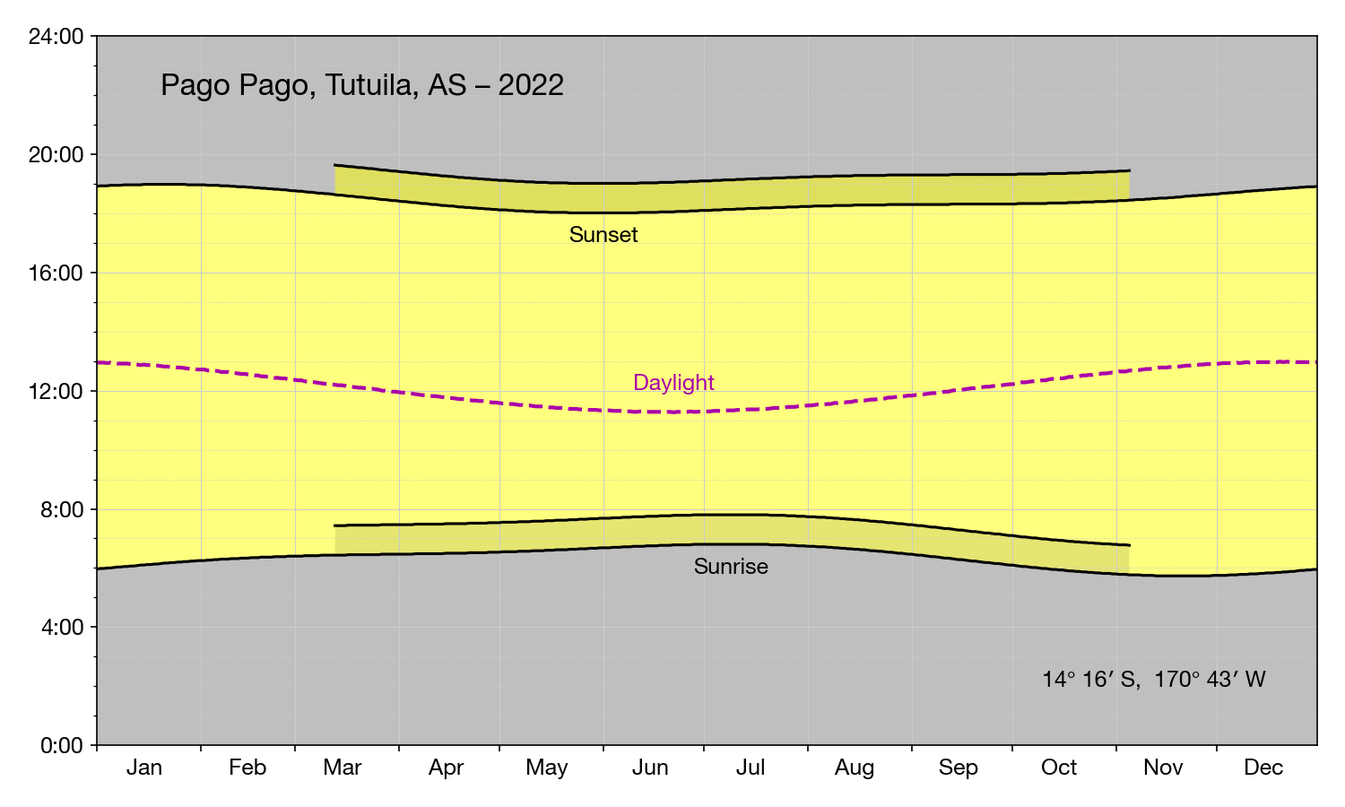
Another interesting thing about these labels is that while the earliest sunrise, latest sunset, and longest daylight occur near the middle of the year for most of the US, there’s a place where that is reversed. American Samoa is in the southern hemisphere, so if I used the same label-positioning rules for it as I used for the rest of the country, the labels would be off at one end of the year or the other and might run off the end of the plot. So Lines 165–182 account for that by determining whether we search for peaks or valleys depending on the N or S at the end of the latitude string. For example, here’s a plot for Pago Pago:

They don’t use DST in Pago Pago; it’s too close to the equator for DST to be useful, and the US rules would make the adjustments go in the wrong direction. But I’m plotting it anyway—just as I plot it for Phoenix, Honolulu, and other places that don’t use DST—to show how the rules would work if they were applied. I’m showing Standard Time in the summer for places that switch to DST, so it seems consistent to show DST even in places where it doesn’t apply.
I’ve thought about adding a dashed line showing where DST would be in the winter months. Last year, the Senate passed a bill for year-round DST (the House let it lie), so it might be nice to show the consequences of that graphically. But for now, I’m going to put this away and move on to other ways of wasting my time.
Update 11 Nov 2023 4:32 PM
Based on a tip from Marcos Huerta, I watched this video from Jacqueline Nolis and realized I have more work ahead if I expect to handle places in Alaska. Go to the USNO site and request data for Nome, AL. What a mess! Starting in late May, the sunsets are so late they roll over past midnight into the next day. From then until mid-July, a naive reading of the data (which is what my code does) says that sunset comes before sunrise. This year, and probably most years, there’s a day in mid-July with two sunsets, one just after the midnight at the beginning of the day and another just before the midnight at the end of the day. July 17, the day in question, has two lines associated with it.
Ms. Nolis, who’s pulling this same data from another online source and is using R to plot it, suggests using three days of data for each being plotted—the day before, the day of, and the day after—and then truncating the plot to show only the day of. That seems like a reasonable approach, but it may not be so reasonable if I continue to use the USNO data. I’ll have to give it some thought.
One thing I’m sure of is that I want to stick with Python and Matplotlib instead of switching to R. I’ve done enough with R to know that its syntax is not for me, no matter how appealing Kieran Healy makes it seem.
