Processing layered SVGs
February 15, 2020 at 9:54 PM by Dr. Drang
Over the past few months, I’ve been creating and processing a lot of SVG files. Initially, the processing was mostly manual, via cutting, pasting, finding, and replacing in BBEdit. But I’ve gradually learned how to use Python’s XML modules to automate the processing, which has both sped up my work and increased its accuracy.
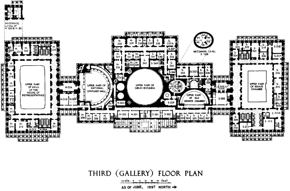
Most of my work has started with me tracing over the areas of interest in plan view drawings so I can calculate distances and areas. The drawings usually come to me as bitmapped images1 like this one of the US Capitol, which I downloaded from Wikipedia.

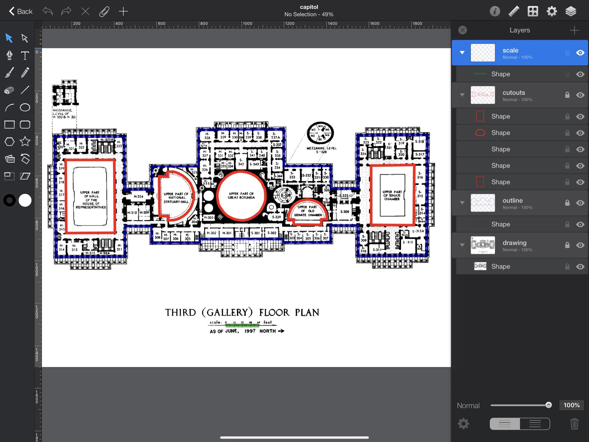
Let’s say I want to get the area of this floor. I start by importing the file into a vector graphics program like Graphic, OmniGraffle, or Affinity Designer. Then I make layers above the bitmap and draw in the outer boundary, the holes or cutouts in the floor, and some length or feature that I can use to scale the drawing. Here’s what it looks like in Graphic on the iPad.

You can see the layers to the right of the image. The drawing layer is for the bitmap, the outline layer is for the outer boundary in blue; the cutouts layer is for the open areas of the Rotunda, the House and Senate chambers, the old Senate chambers, and Statuary Hall outlined in red; and the scale layer is for the green box drawn over the 64-foot scale just below the title.
I’ve made this graphic higher in resolution than I normally do for images here so you can zoom in to see the structure if you like. If you do, you’ll notice that the curved areas of the cutouts are approximated by a series of straight lines. I could have used Bezier curves for those portions, but straight lines work better with the Shapely library, which is what I’m going to use to calculate the area (in the next blog post; this one is going to concentrate on processing the SVG, which I’m about to get to).
So now I have a document in Graphic’s native format, which doesn’t do me much good. What I need to do next is export it as an SVG file, which, conveniently, Graphic can do on both the Mac and iPad. What comes out is a very large text file that looks like this:
xml:
<?xml version="1.0" encoding="UTF-8"?>
<!DOCTYPE svg PUBLIC "-//W3C//DTD SVG 1.1//EN" "http://www.w3.org/Graphics/SVG/1.1/DTD/svg11.dtd">
<svg version="1.1" xmlns="http://www.w3.org/2000/svg"
  xmlns:xlink="http://www.w3.org/1999/xlink" x="0" y="0" width="2000" height="1500"
  viewBox="0, 0, 2000, 1500">
  <g id="Background">
    <rect x="0" y="0" width="2000" height="1500" fill="#FFFFFF"/>
  </g>
  <defs>
    <clipPath id="Clip_1">
      <path d="M80.5,144.5 L1919.5,144.5 L1919.5,1355.5 L80.5,1355.5 z"/>
    </clipPath>
  </defs>
  <g id="drawing">
    <image
      xlink:href="data:image/png;base64,iVBORw0KGgoAAAANSUhEUgAABy8AAAS7CAIAAACnxmE+A

      [lots and lots of base64 snipped out]

      ECBAgAABAgQIECBAgAABAgQIENhd4P8DXwQCGxoPV+EAAAAASUVORK5CYII="
      opacity="1" x="80.5" y="144.5" width="1839" height="1211"
      preserveAspectRatio="xMidYMid" clip-path="url(#Clip_1)"/>
  </g>
  <g id="outline">
    <path d="M123.599,412.613 L446.663,412.9 L452.08,664.029 L578.999,662.481
      L579.773,552.975 L796.461,552.575 L797.666,380.968 L1200.281,379.81
      L1199.042,551.939 L1420.726,551.234 L1422.843,657.932 L1547.177,658.461
      L1547.066,407.545 L1876.229,404.746 L1872.399,972.508 L1548.302,975.134
      L1547.528,831.19 L1419.062,831.19 L1419.448,910.514 L1195.406,911.675
      L1195.793,895.036 L803.041,895.423 L803.815,912.836 L579.367,914.412
      L577.414,836.858 L453.829,837.974 L452.992,978.854 L124.207,981.041
      L123.599,412.613 z" fill-opacity="0" stroke="#0000FF" stroke-width="12"
      stroke-opacity="0.518" id="Shape"/>
  </g>
  <g id="cutouts">
    <path d="M173.197,526.183 L401.5,526 L404.38,869.031 L175.5,870.5 z"
      fill-opacity="0" stroke="#FF0000" stroke-width="12"/>
    <path d="M677.405,581.473 L701.206,587.925 L724.173,600.382 L743.054,615.953
      L759.793,635.807 L769.33,658.19 L775.753,680.185 L776.142,709.575
      L769.33,733.516 L760.377,755.121 L743.248,776.532 L725.536,791.714
      L702.374,803.976 L679.406,809.815 L654.687,810.594 L654.687,789.962
      L614.591,789.962 L614.172,600.618 L650.926,600.486 L650.753,581.647
      L677.405,581.473 z" fill-opacity="0" stroke="#FF0000" stroke-width="12"/>
    <path d="M1005.316,580.723 L1024.764,584.138 L1043.23,589.835 L1059.928,598.479
      L1075.054,608.89 L1087.037,621.659 L1096.663,633.249 L1103.342,648.965
      L1110.218,663.305 L1112.182,677.449 L1113.164,694.933 L1113.361,709.273
      L1110.807,723.221 L1103.735,741.294 L1094.699,757.992 L1084.483,773.118
      L1070.339,784.905 L1057.767,794.138 L1043.426,801.603 L1027.121,807.692
      L1012.192,810.594L998.244,810.594 L983.314,808.675 L966.813,804.942
      L949.919,797.87 L934.399,789.227 L918.684,774.886 L908.862,761.921
      L898.646,747.384 L891.574,732.847 L889.021,717.721 L886.86,703.969
      L886.467,692.969 L887.449,678.628 L892.557,661.537 L899.039,641.696
      L907.29,628.927 L919.666,614.587 L933.614,602.211 L947.168,593.764
      L961.705,586.692 L976.832,582.763 L987.44,580.723 L1005.316,580.723 z"
      fill-opacity="0" stroke="#FF0000" stroke-width="12"/>
    <path d="M1221.709,806.373 L1222.147,790.763 L1225.794,776.028 L1232.213,760.419
      L1240.383,747.581 L1250.157,735.91 L1263.141,726.865 L1276.416,719.716
      L1289.108,715.923 L1302.238,713.443 L1313.471,712.568 L1325.58,713.881
      L1337.396,716.507 L1348.338,720.592 L1360.009,725.114 L1371.242,732.846
      L1379.703,741.453 L1386.852,750.644 L1393.271,761.44 L1398.814,773.111
      L1401.44,784.781 L1402.316,792.805 L1403.483,805.643 L1377.223,805.497
      L1375.473,831.757 L1246.51,830.444 L1245.926,806.518 L1221.709,806.373 z"
      fill-opacity="0" stroke="#FF0000" stroke-width="12"/>
    <path d="M1611.074,553.144 L1814.482,549.597 L1811.978,833.534 L1611.32,831.757
      L1611.074,553.144 z" fill-opacity="0" stroke="#FF0000" stroke-width="12"/>
  </g>
  <g id="scale">
    <path d="M927.108,1295.893 L1081.541,1295.893 L1081.541,1313.799 L927.108,1313.799 z"
    fill="#008100" fill-opacity="0.588"/>
  </g>
</svg>
I’ve redacted most of the data associated with the bitmapped drawing, and I’ve added hard line breaks to make it easier to read. In the original, for example, each of the <path> elements is just one long line.
As you can see, each of the layers is inside a <g> element, and the id attribute is the layer’s name. The individual boundaries are <path> elements, and the coordinates of their vertices are inside the d attribute.
If you’ve ever programmed in PostScript or similar graphical languages, the d attributes might look familiar. The M is equivalent to PostScript’s moveto command, the L is like lineto, and the Z is like closepath.2
To prepare for analysis by the Shapely library, I want to pull out all the vertex coordinates and write them out into CSV files. There will be a CSV file for each of the boundaries, and each line of a CSV file will be the x, y coordinates of a vertex. Here’s the code that does it:
python:
 1:  import xml.etree.ElementTree as et
 2:  import re
 3:
 4:  def path2csv(path):
 5:    '''Transform an SVG path into vertex coordinates for a CSV file.
 6:
 7:    The path must consist of only moveto (M) and lineto (L)
 8:    commands with an optional closepath (Z) at the end.'''
 9:
10:    pstr = path.get('d')
11:    # Delete the starting moveto command
12:    pstr = re.sub(r'^M *', '', pstr)
13:    # Delete the closepath command
14:    pstr = re.sub(r' *[zZ]$', '', pstr)
15:    # Put all the vertex points on separate lines
16:    pstr = re.sub(r' *L *', '\n', pstr)
17:    # Separate the x and y coordinates with a comma only
18:    pstr = re.sub(r' +, +| +,|, +| +', ',', pstr)
19:    # Return the multiline string of comma-separated coordinates
20:    return pstr
21:
22:  # Parse the SVG file and get the root
23:  tree = et.parse('capitol.svg')
24:  svg = tree.getroot()
25:
26:  # Handle the outline layer
27:  layer = svg.find('.//{http://www.w3.org/2000/svg}g[@id="outline"]')
28:  opath = layer.find('.//{http://www.w3.org/2000/svg}path')
29:  f = open('outline.csv', 'w')
30:  f.write('x,y\n')
31:  f.write(path2csv(opath))
32:  f.close()
33:
34:  # Handle the cutouts layer
35:  layer = svg.find('.//{http://www.w3.org/2000/svg}g[@id="cutouts"]')
36:  cpaths = layer.findall('.//{http://www.w3.org/2000/svg}path')
37:  for i, p in enumerate(cpaths):
38:    f = open(f'cutout-{i+1:02}.csv', 'w')
39:    f.write('x,y\n')
40:    f.write(path2csv(p))
41:    f.close()
42:
43:  # Handle the scale layer
44:  layer = svg.find('.//{http://www.w3.org/2000/svg}g[@id="scale"]')
45:  spath = layer.find('.//{http://www.w3.org/2000/svg}path')
46:  f = open('scale.csv', 'w')
47:  f.write('x,y\n')
48:  f.write(path2csv(spath))
49:  f.close()
The module we’ll use for parsing and traversing the SVG is xml.etree.ElementTree, imported as et on Line 1. This treats the SVG as a tree structure, with the elements of the document acting as nodes. Lines 23 and 24 read in the SVG file and parse it, leaving us with the root element of the tree saved in the svg variable. We can now traverse down the tree from svg3 to find the data we’re looking for.
The next three sections of the script deal with each layer of drawing—apart from the bitmap layer—in turn. Starting with the outline layer, we
- Find the first (and only)
<g>element in the tree that has anidattribute ofoutline. We’re using XPath syntax to define the query passed to thefindcommand. The query starts at the current node (.) and searches at all levels below it (//) for agnode with the desiredid([@id="outline"]). The URL in curly braces is the XML namespace that defines the structure of an SVG. You can see it as one of thexmlnsattributes of the<svg>root node. - Once we have the
outlinelayer, we search it to find the first (and only)path. The XPath syntax is similar to what we used to find theoutlinelayer. - We then create a CSV file and write the path’s
ddata to it. The data is formatted through thepath2csvfunction defined on Lines 4—20.
These three steps are then repeated to handle the cutouts and scale layers. The only difference is that cutouts has more than one <path>, so we have to use findall instead of find and then loop through all the paths.4 I suppose I should have refactored these stanzas into a single function that gets called repeatedly.
I skipped over the path2csv function because I think it’s pretty easy to follow. Basically, it pulls out the d string from the supplied path and applies a series of regular expression substitutions to make a series of text lines with comma-separated coordinates. The trickiest part is that the syntax for d can vary a bit with regard to spaces and commas. I’ve tried to cover the variations I know about and end up with a consistent CSV format. The outline.csv file, for example, looks like this:
x,y
123.599,412.613
446.663,412.9
452.08,664.029
578.999,662.481
579.773,552.975
796.461,552.575
797.666,380.968
1200.281,379.81
1199.042,551.939
1420.726,551.234
1422.843,657.932
1547.177,658.461
1547.066,407.545
1876.229,404.746
1872.399,972.508
1548.302,975.134
1547.528,831.19
1419.062,831.19
1419.448,910.514
1195.406,911.675
1195.793,895.036
803.041,895.423
803.815,912.836
579.367,914.412
577.414,836.858
453.829,837.974
452.992,978.854
124.207,981.041
123.599,412.613
OK, so now we have a series of CSV files with the boundary coordinates given in pixels (or points, depending on which graphics software was used to create the SVG). The next step is to use the Pandas and Shapely libraries to do the analysis. That’ll be next time.
-
If they came as CAD drawings, the dimensions would be immediately available and I wouldn’t need to go through this rigmarole. ↩
-
OK, the
Zdoesn’t look likeclosepathat all, butCwas already taken forcurveto. ↩ -
Computer scientists live in a world in which trees have their roots at the top. This explains a lot about how computers work. ↩
-
The output file names for the cutouts include a sequential number to distinguish between them. The
i+1in Line 38 accounts for the fact that computer scientists like to start counting at zero instead of one. I don’t know if this is related to their trees being upside down. ↩
