Simple drawings with Mathematica
September 15, 2023 at 6:24 PM by Dr. Drang
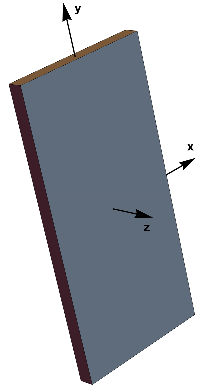
A couple of days ago, I wrote a post that included this image:

Because I don’t have a 3D drawing app, I did it in Mathematica. And because I’m new to Mathematica, I fumbled around a bit before figuring out what to do. I decided to write up what I learned so I could refer to it later, and I decided to post it here in case it’s of any value to anyone else.
The key function when creating 3D images (that aren’t plots) is Graphics3D. As you can see from the linked documentation, it can take an enormous number of arguments and options. The main argument is a list of the objects to be drawn, which in the drawing above consisted of the boxy representation of an iPhone and three arrows representing the x, y, and z axes (I added the axis labels “by hand” in Acorn).
One of the first things I learned was to create the objects separately instead of trying to build them within the call to Graphics3D. It’s certainly possible to make this image entirely within Graphics3D, but the function call becomes really long and confusing if you do it that way. I started by defining variables with the dimensions of the phone (in millimeters):
b = 71.5
h = 147.5
t = 7.85
In case you’re wondering, b is commonly used in my field for the width of objects—it’s short for breadth. We avoid w because we like to use it for weight.
The boxy iPhone is defined using the Cuboid function:
phone = Cuboid[{-b/2, -h/2, -t/2}, {b/2, h/2, t/2}]
The two arguments are its opposite corners.
In theory, I could use Mathematica’s own knowledge of its coordinate system to draw the axes, but it defaults to drawing axes along the edges of a box that encloses the object, and I didn’t find any handy examples of overriding that default. It was easier to define the axes using the Arrow function:
xaxis = Arrow[{{0, 0, 0}, {b/2 + 25, 0, 0}}]
yaxis = Arrow[{{0, 0, 0}, {0, h/2 + 25, 0}}]
zaxis = Arrow[{{0, 0, 0}, {0, 0, t/2 + 25}}]
The argument to Arrow is a list of two points: the “from” point and the “to” point. As you can see, each arrow starts at the origin (which is the center of the phone) and extends in the appropriate direction 25 mm past the edge of the phone. Why 25 mm? It looked about right when I tried it.
With the objects defined, I called Graphics3D to draw them:
Graphics3D[{Gray, phone, Black, Thick, xaxis, yaxis, zaxis},
Boxed -> False, ImageSize -> Large]
(I’ve split the command into two lines here to make it easier to read, and I’ll do the same from now on.)
As you can see, the list of objects that makes up the first argument is interspersed with directives on how those objects are to be drawn. The first directive, Gray, applies that color to phone. Then Black overrides Gray and is applied to the three axes that follow. I added the Thick directive before the axes when I saw that they looked too spindly by default.
The Boxed->False option stops Mathematica from its default of including a wireframe bounding box in the image. ImageSize->Large does what you think—it makes the image bigger than it otherwise would be.
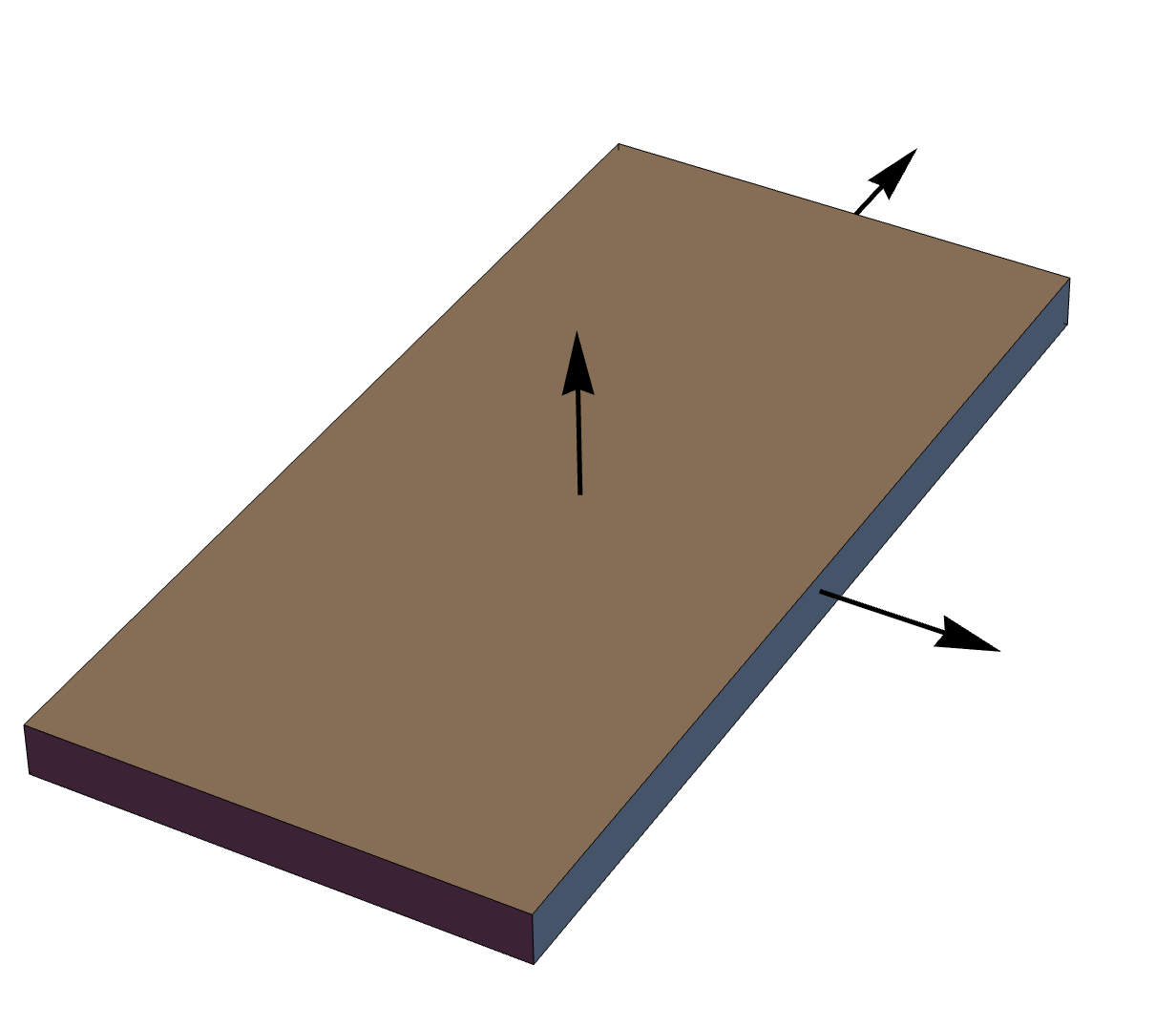
Here’s what Mathematica displays:

Mathematica obviously thinks the z direction should be pointing up. This makes sense, but it isn’t what I wanted. The notebook interface allows you “grab” the image and rotate it into any orientation, so that’s what I did, putting it into the position you see at the top of the post. Then I right-clicked on the image and selected from the contextual menu. I opened the resulting image file in Acorn, added the axis labels, and uploaded the result to my web server.
After publishing the post, I returned to Mathematica to see if I could get it to clean a few things up. First, I wasn’t happy with the brownish color that appeared on certain edges, depending on the orientation. That was cleared up with the Lighting->Neutral option. Then I wanted programmatic control over the orientation, which I got via ViewPoint->{-50, 30, 75}, which sets the location of the virtual camera, and ViewVertical->{.1, 1, 0}, which rotates the camera about the axis of its lens until the given vector is pointing up in the image.
Finally, I wanted to add the axis labels in Mathematica instead of relying on another program. This meant adding Text objects to the argument list, one for each axis. The final call to Graphics3D looked like this:
Graphics3D[{GrayLevel[.5], phone,
Black, Thick, xaxis, yaxis, zaxis,
FontSize -> 16,
Text["x", {b/2 + 25, -7, 0}],
Text["y", {-7, h/2 + 25, 0}],
Text["z", {-5, -5, t/2 + 25}]},
Boxed -> False, ImageSize -> Large,
ViewPoint -> {-50, 30, 75}, ViewVertical -> {.1, 1, 0},
Lighting -> "Neutral"]
Each Text object includes both the text and the point at which it is to be displayed. The Text items are preceded by a FontSize directive to make them big enough to see clearly. The Black directive earlier in the list was still in effect, so the text color was black.
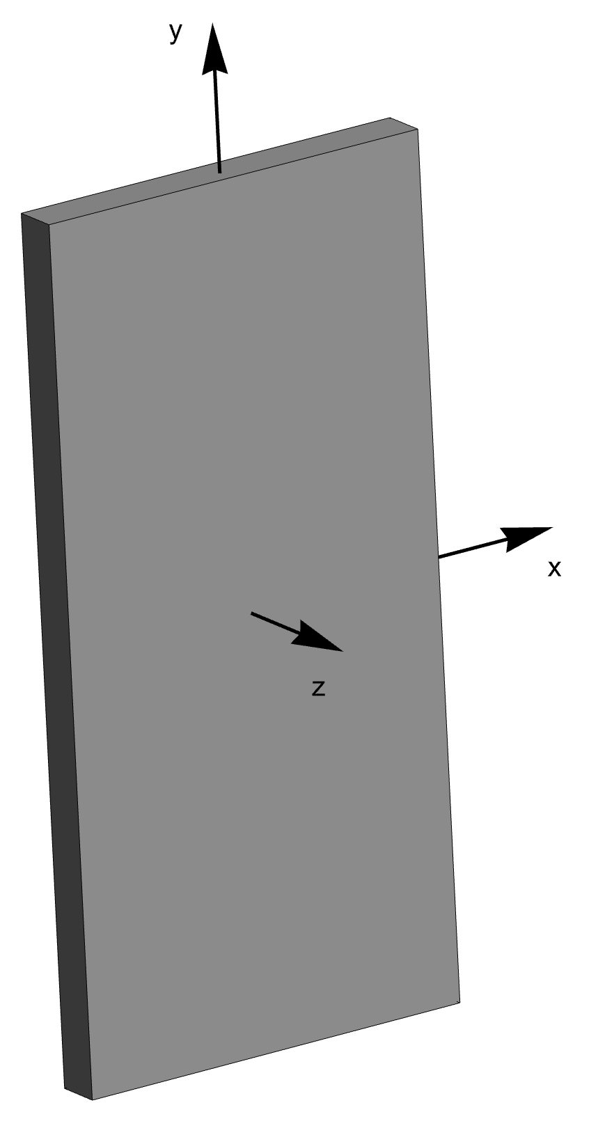
Here’s the result:

As you can see, I’ve made the image more upright, and the neutral lighting has gotten rid of the weird brownish and bluish casts of the original. You may also note that I changed the original Gray directive to GrayLevel[.5]. This made no difference in the final output, but the GrayLevel argument did let me play around with different shades of gray before deciding that the 50% provided by Gray was just fine.
I still have a long way to go with Mathematica, but I’m making progress.
