Moment diagrams for simply supported beams
April 3, 2024 at 3:33 PM by Dr. Drang
I thought I’d run through how the moment diagrams in the last post were made. It’ll probably take two articles to get through it all.
Let’s start with the three simple spans.
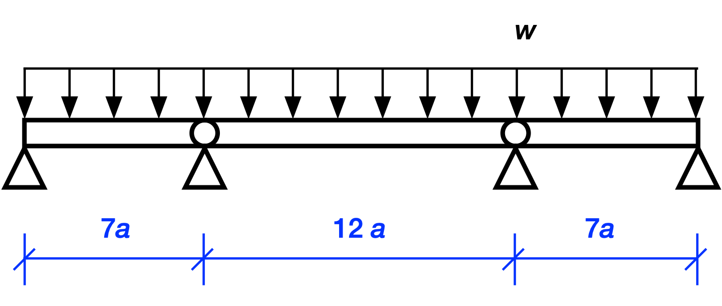
We’ll generate the moment diagram for a single simply supported beam and then apply it to each individual span.
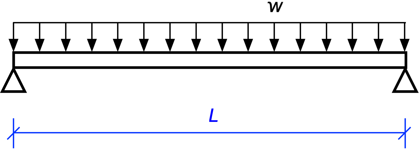
Note here that is the uniform intensity of the load along the beam. It can be measured in pounds per foot, kilonewtons per meter, or any units that work out to force per length. The total load on beam is .
We start by drawing the free body diagram for the beam, replacing the supports with their associated reaction forces.
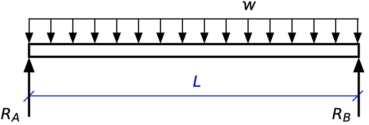
There are two unknowns, and , and two equations of statics:1
The first represents the sum of all the forces in the vertical direction, and the second represents the sum of all the moments about the left end of the beam (Point A). The solution to these two equations is
You could have gotten this same answer with no algebra by taking account of symmetry. Because the structure is symmetric and the loading is symmetric, the reaction forces must also be symmetric.2 (I guess there’s a little algebra because you need to know that the two equal reactions add up to , but that really doesn’t count, does it?)
With the reaction forces determined, we move on to determining the bending moment within the beam. When a structure is in equilibrium, every portion of it is in equilibrium. So we can consider just part of the beam, a section of length starting at the left end, and draw its free body diagram:
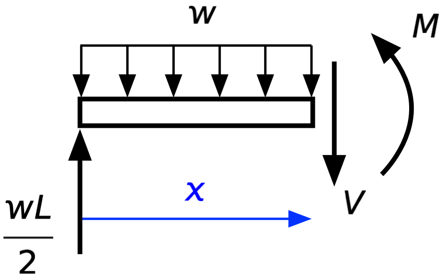
Because we have conceptually cut the beam at a distance from the left end, we’ve exposed the internal shear, , and moment, , and can write the equations of statics for this portion of the beam.
In the second equation, we’re taking moments about the right end of this portion.
Solving these two equations gives us
and
Although the shear matters in beam design, the moment is typically more important, so we’ll focus on that. The equation for is that of a parabola, with at and and rising to a peak of
at midspan, .
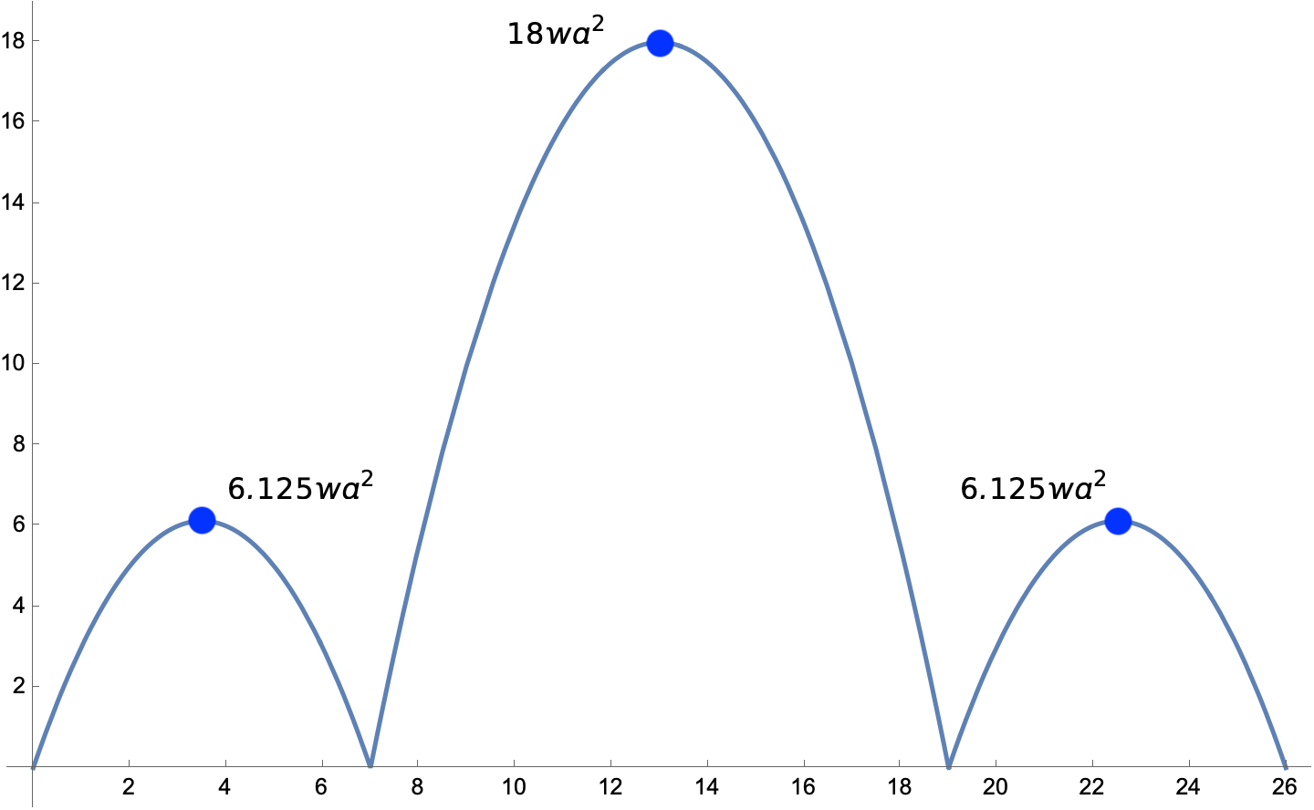
For the middle span of the three-span bridge, , so
at its center. And for the two side spans, , so
at their centers. These are the labeled dots in the moment diagram at the top of the post.
To make the moment diagram in Mathematica,3 we have to start by taking the generic equation for and rewriting it as three equations that work in the individual spans, where the origin of the coordinate is at the left end. That will look like this:
To get Mathematica to plot this, we need to nondimensionalize the moment and the horizontal coordinate so we’re plotting pure numbers, with no or terms left in the expressions. We do that by dividing through by to nondimensionalize and by introducing a new variable, , to nondimensionalize the horizontal coordinate. That gives us
Now we’re ready to move to Mathematica for the plotting.
First, we define three s, one for each span, and then use the Piecewise function within Plot to get a moment diagram that covers all three spans:
    m1 = 1/2*u*(7 - u);

    m2 = (u - 7)/2*(12 - (u - 7));

    m3 = (u - 19)/2*(7 - (u - 19));

    Plot[Piecewise[{{m1, u <= 7}, {m2, 7 < u <= 19}, {m3, u > 19}}],
     {u, 0, 26},
     ImageSize -> Large,
     PlotStyle -> Thick,
     Ticks -> {Table[t, {t, 0, 18, 2}], Table[t, {t, 0, 26, 2}]}]
That gives us the moment diagram shown at the top of the post, except for the dots and the labels at the peaks of the parabolas. I added those “by hand” in Preview.
Simply supported beams are called “statically determinate” structures because we can determine all the internal and external forces through statics alone. That won’t be the case for the three-span continuous beam, which we’ll analyze in the next post.
-
Normally there would be three equations of statics for a plane problem like this, but because there are no forces in the horizontal direction, the horizontal equilibrium equation gives us no information. It’s just 0 = 0. ↩
-
“Symmetric” here means symmetric about the midspan of the beam. In other words, the right half of the beam is a mirror image of the left half. ↩
-
I could’ve plotted it with Python and Matplotlib, but I want to learn more about Mathematica, so I used this as an opportunity to do so. ↩
