And now it’s all this

I just said what I said and it was wrong
Or was taken wrong

Next post Previous post

Random points without rejection

May 10, 2025 at 9:20 AM by Dr. Drang

A few days ago, John D. Cook wrote a post about generating random points on the surface of a sphere. His approach was:

1. Generate three independent uniformly distributed random variables in the range from $-R$ to $+R$, where $R$ is the radius of the sphere. These will represent a point in $(x,y,z)$ space.
2. Calculate $S$ such that $$S^2=x^2+y^2+z^2$$
3. If $S>R$, which means the point is outside the sphere, reject the point and go back to Step 1.

4. Otherwise, return the point

   $$(\frac{x}{S},\frac{y}{S},\frac{z}{S})$$

   which is a projection of the point out onto the surface of the sphere.

This works, of course, but you reject nearly half of the points you generate. All the points are in a cube of volume $8R^3$, but you’re keeping only those in a sphere of volume $\frac{4}{3}\pi R^3\approx 4.19R^3$

I wanted to come up with a way to generate points directly on the sphere without any rejections or projections. To start, I decided to reduce the problem by one dimension and think about circles.

Generating random points around the circumference of a circle is pretty easy. Just generate a series of uniformly distributed random variables from $0$ to $2\pi$ and treat them as angles, ${\theta }_i$. Then the points $(R,{\theta }_i)$ will be distributed around the circumference. Like this:

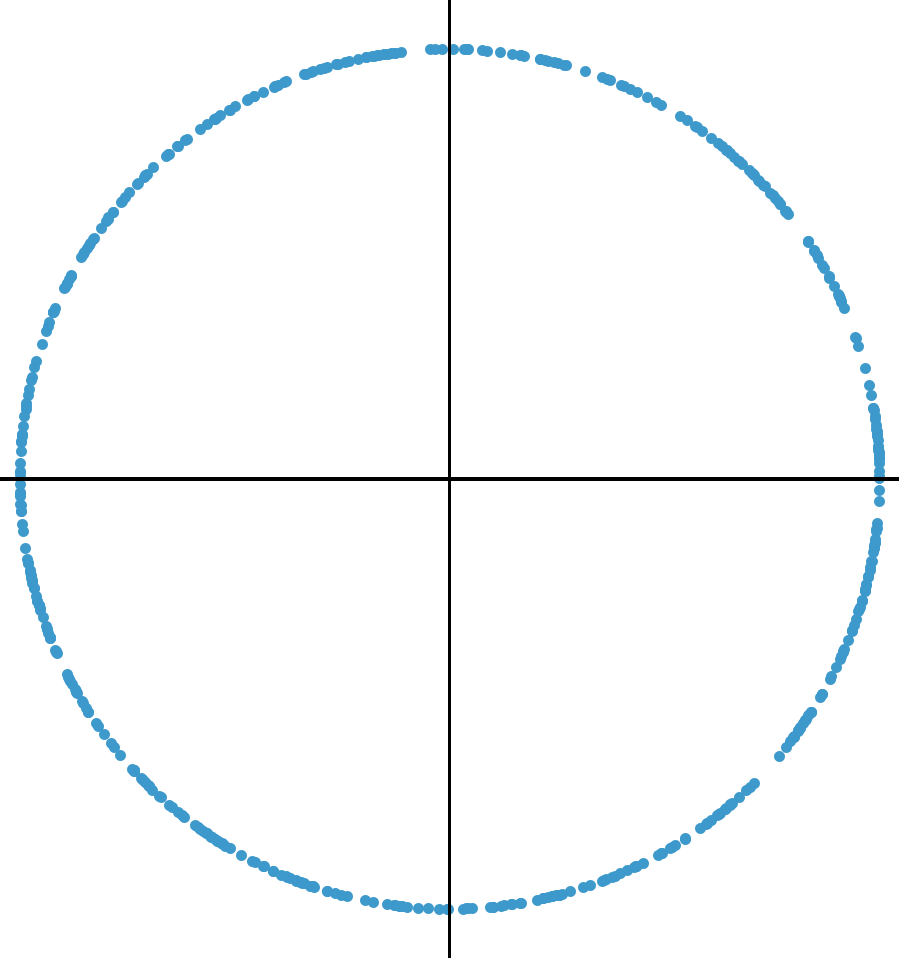
This is 500 points, and there are some gaps and clumps because that’s the nature of random number generation. But there’s no bias to the distribution of points.

Now let’s generate points within the circle. A naive way to go about this would be to generate values uniformly distributed between $0$ and $2\pi$ for the angle, as before, and to generate values uniformly distributed between $0$ and $R$ for the radius. But if we do that, we’ll get a point cloud of $(r_i,{\theta }_i)$ pairs that looks like this:

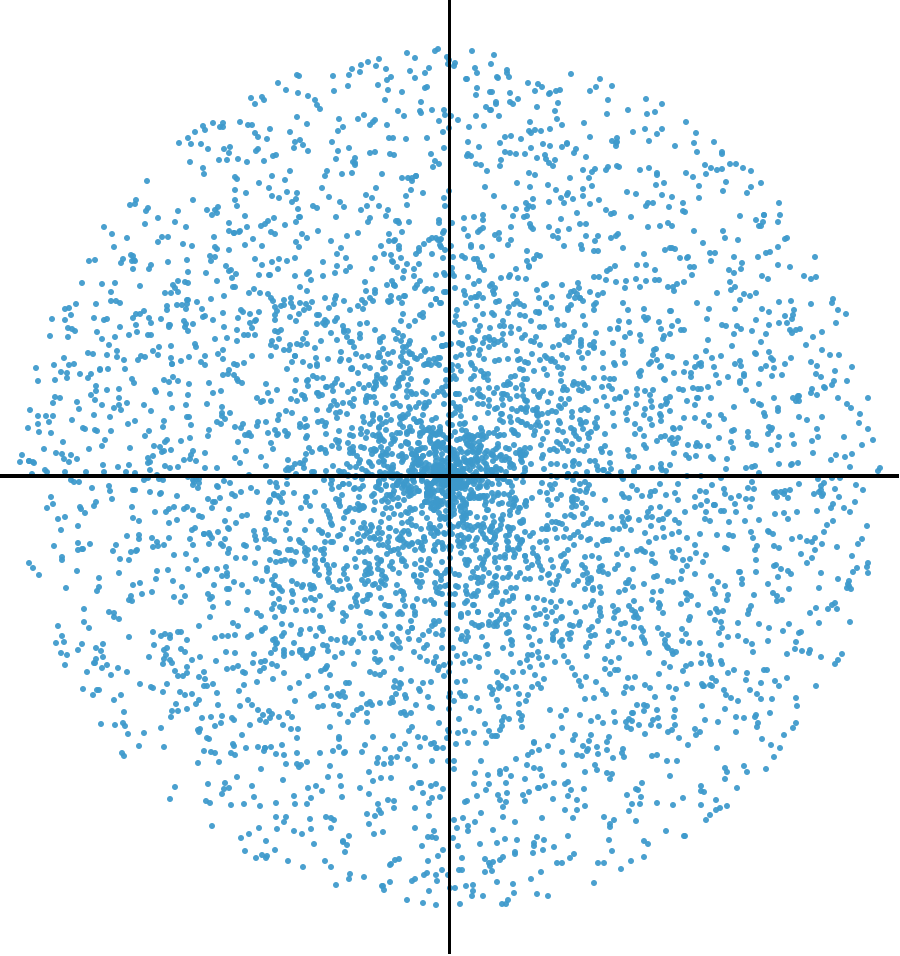
Definitely biased toward the center of the circle.

Why did this happen? Consider this polar grid:

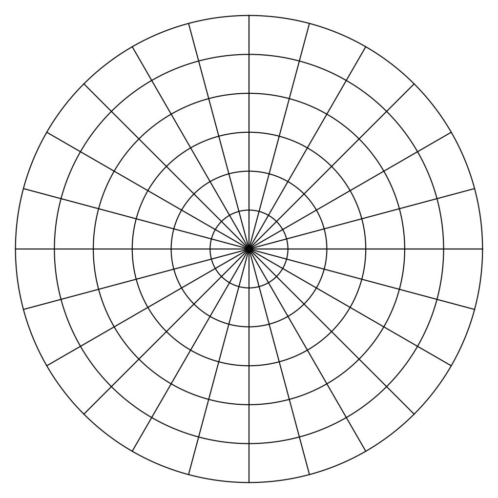
If we generate uniformly distributed $r_i$ and ${\theta }_i$, all the sectors in the grid will have about the same number of points. But because the sectors near the center are smaller, the points will be denser in those sectors and sparser in the sectors further out. Which is exactly what we see in the naive point cloud.

The size of the sectors grows linearly with $r$, so we need to generate the $r_i$ using a distribution that grows linearly with $r$. That would be a triangular distribution with a probability density function that looks like this (for $R=5$):

The peak value of the PDF is $\frac{2}{R}$ because the area under the PDF must be one.

Many math software packages have functions for generating random variables with a triangular distribution. Using that distribution instead of a uniform distribution for generating the $r_i$ will give us a set of $(r_i,{\theta }_i)$ that’s uniformly spread over the interior area of the circle:

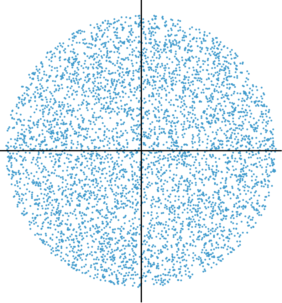
How did I know to use a triangular distribution for $r$? The polar grid certainly shows that we need to generate more large $r$ values than small ones, but how did I know that a PDF with linear growth was the one to use? There are, I suppose, many ways to think about the problem, but I thought of it in terms of the Jacobian, a topic you typically learn about in a multivariable calculus class.

We know that in Cartesian coordinates, a differential area element is the product of the two differential linear elements:

$$dA=dxdy$$

But in polar coordinates, the expression for differential area is a little more complicated:

$$dA=rdrd\theta$$

We can get this expression by considering the equations that convert between polar and Cartesian coordinates:

$$\begin{array}{c}x=r\cos \theta \hfill \\ y=r\sin \theta \hfill \end{array}$$

The differentials are

$$\begin{array}{c}dx=\cos \theta dr-r\sin \theta d\theta \hfill \\ dy=\sin \theta dr+r\cos \theta d\theta \hfill \\ \hfill \end{array}$$

which can also be expressed in matrix form:

$$\left\{\begin{array}{c}\hfill dx\hfill \\ \hfill dy\hfill \end{array}\right\}=\left[\begin{array}{cc}\hfill \cos \theta & \hfill -r\sin \theta \\ \hfill \sin \theta & \hfill r\cos \theta \end{array}\right]\left\{\begin{array}{c}\hfill dr\hfill \\ \hfill d\theta \hfill \end{array}\right\}$$

The determinant of the matrix (called the Jacobian) represents the ratio of the differential areas expressed in the two coordinate systems:

$$dxdy=\left|\begin{array}{cc}\hfill \cos \theta & \hfill -r\sin \theta \\ \hfill \sin \theta & \hfill r\cos \theta \end{array}\right|drd\theta =rdrd\theta$$

That $r$ in the expression tells us that we need to scale linearly with $r$. Hence the triangular PDF with the shape given above.

OK, now it’s time to move from circles to spheres. Here’s our coordinate system:

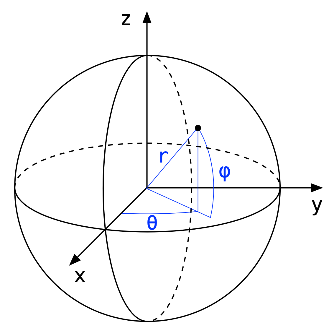
There are different ways to define the two angles. I’ve chosen a system where $\theta$ is like longitude and $\varphi$ is like latitude. The relationship between the Cartesian and spherical coordinates is this:

$$\begin{array}{ccc}\hfill x& \hfill =\hfill & r\cos \varphi \cos \theta \hfill \\ \hfill y& \hfill =\hfill & r\cos \varphi \sin \theta \hfill \\ \hfill z& \hfill =\hfill & r\sin \varphi \hfill \end{array}$$

Which means the differential relationship is

$$\left\{\begin{array}{c}\hfill dx\hfill \\ \hfill dy\hfill \\ \hfill dz\hfill \end{array}\right\}=\left[\begin{array}{ccc}\hfill \cos \varphi \cos \theta & \hfill -r\cos \varphi \sin \theta & \hfill -r\sin \varphi \cos \theta \\ \hfill cos\varphi \sin \theta & \hfill r\cos \varphi \cos \theta & \hfill -r\sin \varphi \sin \theta \\ \hfill \sin \varphi & \hfill 0& \hfill r\cos \varphi \end{array}\right]\left\{\begin{array}{c}\hfill dr\hfill \\ \hfill d\theta \hfill \\ \hfill d\varphi \hfill \end{array}\right\}$$

The determinant has lots of trig cancelation, and we end up with

$$dV=dxdydz=r^2\cos \varphi drd\theta d\varphi$$

as the relationship between differential volumes in the two coordinate systems.

Of course, we’re interested in surface area, not volume, but this analysis is still helpful. To get the differential surface area in spherical coordinates, we drop the $dr$ and set $r=R$:

$$dA=R^2\cos \varphi d\theta d\varphi$$

So to get points on a sphere’s surface that are uniformly distributed over the area, $\theta$ is drawn from a uniform distribution from $-\pi$ to $\pi$ and $\varphi$ is drawn from a distribution whose PDF follows a cosine curve from $-\frac{\pi }{2}$ to $\frac{\pi }{2}$:

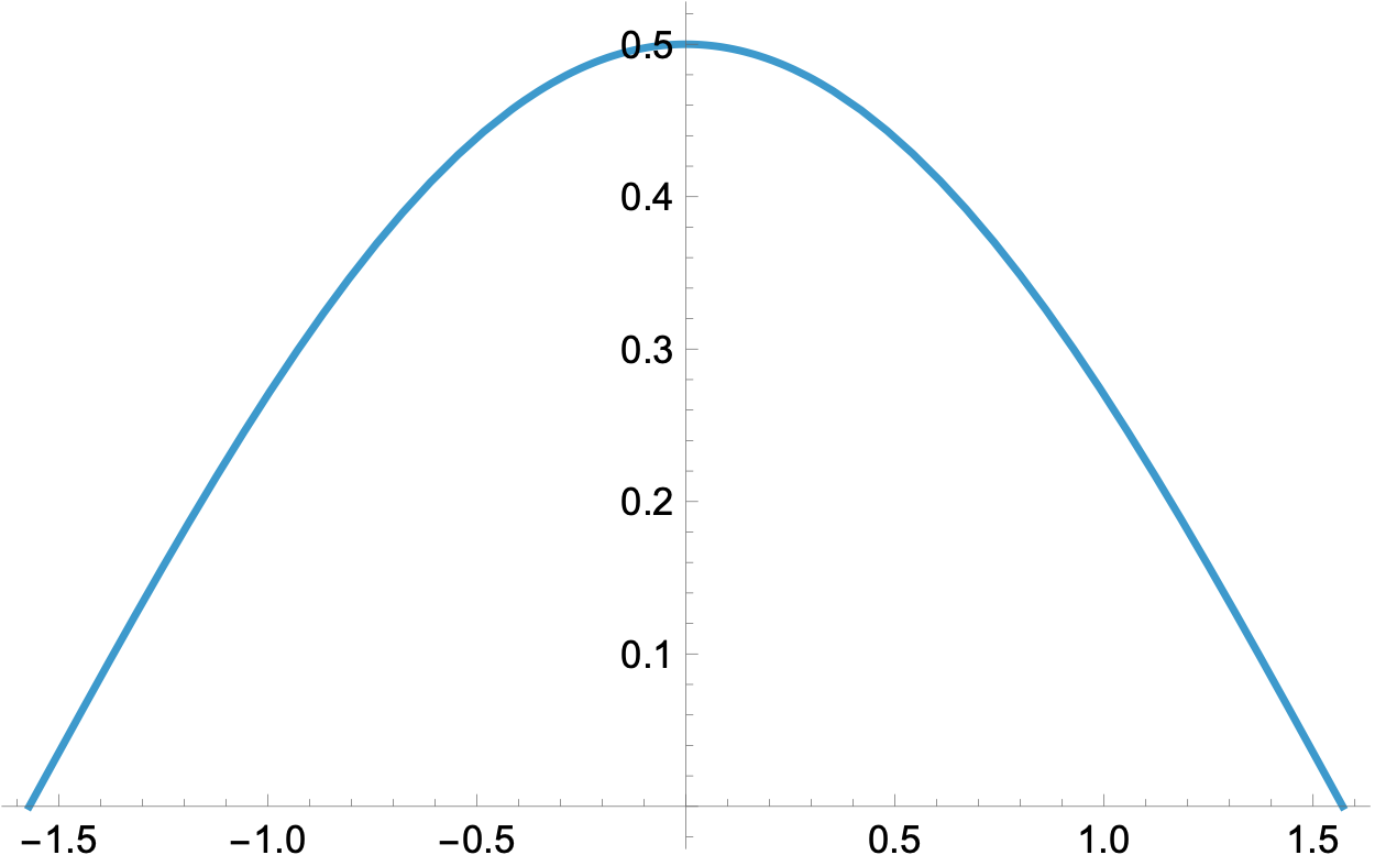
To make this a legitimate PDF, the cosine has been scaled so the integral under the curve is one:

$$f(\varphi )=\frac{\cos \varphi }{2}$$

Unfortunately, this kind of distribution isn’t common. I don’t know of any math packages that include functions for a cosine distribution. No matter. There’s a procedure for generating random numbers from any distribution. We start by integrating the PDF to get the cumulative distribution function:

$$F(\varphi )=\int \frac{\cos \varphi }{2}d\varphi =\frac{\sin \varphi }{2}+C$$

The constant of integration, $C$, is determined by noting that $F=0$ at $\varphi =-\frac{\pi }{2}$. That means $C=\frac{1}{2}$ and

$$F(\varphi )=\frac{1+\sin \varphi }{2}$$

which looks like this:

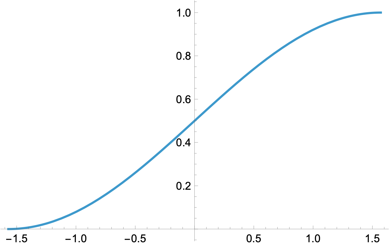
Here’s the trick: CDFs always have a range from zero to one. So if we generate random numbers that are uniformly distributed from zero to one—which is the most common random number generator—and run them through the inverse of the CDF, we’ll get random numbers with the distribution of interest. In this case,

$$F^{-1}(u)=\sin {}^{-1}(2u-1)$$

Here’s the Mathematica code for generating a list of 5000 random points on the surface of a sphere of radius 5:

n = 5000;
R = 5;
\[Phi] = ArcSin[2*RandomReal[1, n] - 1];
\[Theta] = RandomReal[{-Pi, Pi}, n];

And here’s the conversion to Cartesian coordinates:

x = R Cos[\[Phi]] Cos[\[Theta]] ;
y = R Cos[\[Phi]] Sin[\[Theta]];
z = R Sin[\[Phi]];

It actually looks nicer in a Mathematica notebook because the Greek letters are rendered properly:

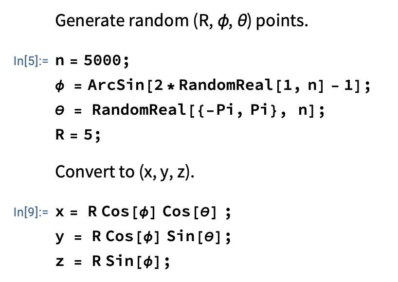
I did this in Mathematica to give me practice. Python code would be similar using NumPy.

Here’s the plot of the randomly generated points:

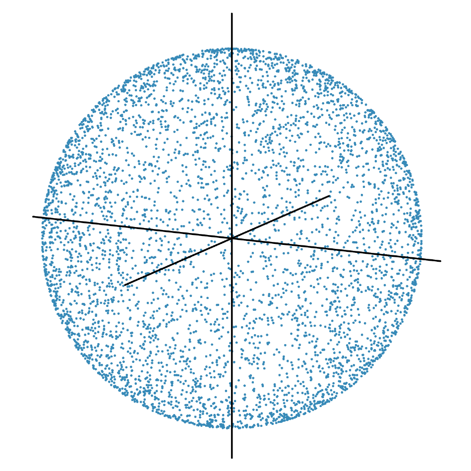
It may not be obvious that the points are on the sphere’s surface. Here’s a video of the point cloud rotating slowly. If you look carefully, you’ll see clumps of points moving from the front surface to the rear and vice versa. There are no points within the sphere to block your view.

Is this a better approach than Cook’s rejection/projection method? I guess that depends on your definition of better. To me, this is a cleaner approach because we’re generating the points on the sphere directly. But random number generation is an inherently numerical procedure, which means efficiency can’t be overlooked. Even though Cook is generating three random numbers for every two I generate—and then thows away nearly half of them—I suspect the simpler numerics of his method will win out. My technique uses a handful of trig functions, whereas his most complicated function is the square root.

But it was a fun problem to think about, and it’s the first time I’ve animated a graph in Mathematica.

Next post Previous post

Site search

Meta

• drdrang at leancrew
• Blog archive
• RSS feed
• JSON feed
• Mastodon
• GitHub repositories

Recent posts

Credits

This work is licensed under a Creative Commons Attribution-Share Alike 3.0 Unported License.

© 2005–2025, Dr. Drang