Barycentric coordinates and random distribution of points
September 11, 2025 at 9:28 PM by Dr. Drang
This morning, John D. Cook posted an article about generating uniformly distributed points over the interior of a triangle. He offered three options, one that failed to distribute the points uniformly and two that succeeded. I want to talk about the failure.
In the failure, he used barycentric coordinates to describe locations within the triangle. These coordinates, which I called area coordinates (because that’s the terminology I learned 40 years ago) in a post written a few years ago are a set of three values in the [0, 1] range, each representing how close the point in question is to one of the triangle’s corners. You can follow the links to get more complete descriptions. One important characteristic of these coordinates is that they are not independent of one another—their sum has to equal one.
Cook’s failed approach (which he knew would fail) consisted of three steps:
- Generate random numbers α, β, and γ from the interval [0, 1].
- Normalize the points to have sum 1 by dividing each by their sum.
- Return αA + βB + γC.
where A, B, and C are the three corner points of the triangle.
He gives an example of randomly generated points and shows that this procedure doesn’t lead to a uniform distribution of the points over the interior of the triangle. But he doesn’t explain why, which is what I spent some time this afternoon exploring.
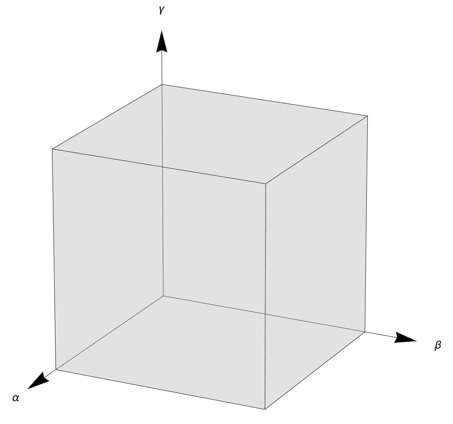
Cook’s first step generates uniformly distributed points in the unit cube that has one of its corners at the origin of the Cartesian coordinate system.

The normalization in the second step creates three new values, , , and , where
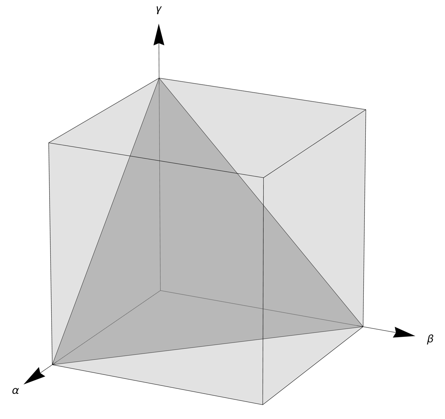
This projects the point onto the plane, which slices through the cube, making a tilted equilateral triangle whose corners are at the (1, 0, 0), (0, 1, 0), and (0, 0, 1) corners of the cube. I’m going to call this the normalization plane.

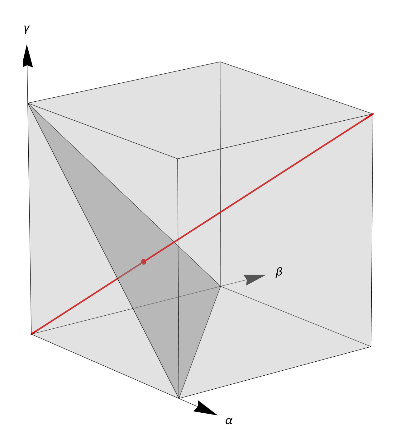
By “projection,” I mean the point is moved along the line defined by the point and the origin until it intersects with the plane. That movement could be either toward the origin or away from it, depending on which side of the normalization plane the original point lies. Here’s a figure that illustrates this idea:

If the point generated in Step 1 lies anywhere on the red line, the normalization in Step 2 will move it to the red dot. I’ve changed the viewing angle so it’s easier to see that the red dot is on the normalization plane.
The line I’ve drawn above, which runs out from the origin to the opposite corner of the cube, is the longest such line that can be drawn. Its length is . The shortest such lines, of which there are three, run out from the origin to the adjacent corner on an axis; they all have lengths of .
The lengths of the lines correspond to the relative likelihood of a point on the normalization plane being generated by the combination of Steps 1 and 2. So a point near the center, as in the image above, is 1.732 times as likely to be generated as a point out near one of the corners. This is how we get nonuniformity in the normalized points even though the original random points are uniform.
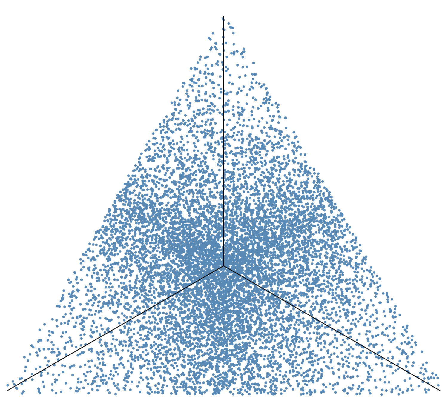
Here’s an illustration. I generated 10,000 points uniformly in the unit cube and normalized them. An isometric view looking toward the origin from the opposite corner of the cube shows the points on the normalization plane distributed like this:

This matches the distribution over an equilateral triangle shown on this MathWorld page, which uses the same procedure we are.1
Cook’s final step is just a distortion of the above equilateral triangle to a more general triangle. If you look at his first figure, it should be pretty obvious how it’s just a squeezed, stretched, and rotated version of the figure above. The main features of the distribution—sparse near the corners, denser at the midsides, and densest at the centroid—are maintained through the distortion.
I suppose I could work out the joint probability distribution of the normalized coordinates using the technique I talked about in this post and this one. But my goal was to understand why the distribution had the pattern it does, not to work out all its mathematical details. Thinking about the line lengths got me there.
-
MathWorld calls them trilinear coordinates instead of barycentric or area coordinates. Varying nomenclature can be fun! ↩
