Port ability
March 10, 2026 at 7:53 PM by Dr. Drang
I read Jason Snell’s review of the MacBook Neo this morning and was struck by this section on its two USB-C ports:
So Apple has done the work to put two USB-C ports on the Neo—and those ports reveal a bit more of the struggles Apple had in building this computer. Both of the USB-C ports will let you charge (which is good, because there’s no MagSafe), but only the one that’s furthest back is a fully functional USB 3 port with support for driving an external display at 4K, 60 frames per second. The closer-in USB port only offers USB 2 speeds. (The good news is that Apple has built alerts into macOS that will warn you if the device you’ve plugged into the slow port would be better off plugged into the faster one, so you won’t be transferring files slowly unnecessarily.)
It reminded me of Christina Warren’s angry Mastodon post about the Neo’s ports:
I’m just going to say that pointing out flaws in $600 and $700 laptops and having people instinctively respond “it’s not for real users, these buyers don’t know/care” is gross. Why should we make the assumption that those buyers don’t still deserve better, or at least on par with the 6 year old product it’s replacing that sold at the same price. Stop assuming people who don’t spend $1000+ on tech are imbeciles or deserve subpar options. No one in 2026 deserves a laptop with a single USB 3 port.
My first thought upon reading Christina’s complaint last week was “Why should I care about the configuration of a computer I’ll never buy?” Kind of a Republican thought, I admit, and I’m not proud of it. But I have many reasons to be disappointed by Apple, and I need to conserve my outrage. Christina’s much younger than I am and has deeper outrage reserves.
Jason pointed out the biggest problem with the low-speed port in his next paragraph:
Honestly, I’m more disappointed by the fact that mismatched ports can lead to user frustration—no, not that port, the other one—than I am about the one slow USB port.
Many Neo users will be too young to remember the joy of flipping USB-A plugs back and forth before getting the orientation right. Apple has updated that wonderful experience for the USB-C age.
Lent and Lisp
February 25, 2026 at 9:13 AM by Dr. Drang
After writing last week’s post about the start of Ramadan and Chinese New Year, I expected to hear from people asking why I didn’t include the further coincidence of Ash Wednesday. I was surprised that the only such feedback I got was an email from TJ Luoma. It makes sense that Lent would be on TJ’s mind—it’s a big part of his business calendar—but I had an answer prepared, and I wrote him back with my reasons.
As I typed out the reply, though, the reasons seemed weaker. Yes, it’s true that the full moon that determines this year’s date of Easter (and therefore Ash Wednesday) isn’t part of the same lunation that determines the start of Ramadan and Chinese New Year, so there was an astronomical reason to keep Ash Wednesday out of the post. But it’s also true that both Ramadan and Lent represent periods of self-denial, so there’s a cultural connection.
Adding a new bit of Emacs Lisp code to what I’d already written to include a check for Ash Wednesday wouldn’t be hard, but another thought was buzzing in my head: switching from Emacs Lisp to Common Lisp. The ELisp calendar functions were written by Edward Reingold and Nachum Dershowitz, authors of the well-known Calendrical Calculations. That book includes a lot of code that isn’t in the Emacs implementation, code that does astronomical calculations I’d like to explore. So it seemed like a good idea to write a Ramadan/Lent/Chinese New Year script in Common Lisp and use the functions from the book.
The problem with that idea was that the Common Lisp code I downloaded from the Cambridge University Press site, calendar.l, didn’t work. I tried it in both SBCL and CLISP, and calling
(load "calendrical.l")
threw a huge number of errors. I was, it turned out, not the first to have run into this problem. The workarounds suggested there on Stack Overflow didn’t help. There’s a port to Clojure that apparently works, but I was reluctant to use Clojure and have to maintain both it and a Java Virtual Machine.
What I found, though, was that Reingold & Dershowitz’s code would load in CLISP with one simple change. After many lines of comments, the working part of calendar.l starts with these lines:
(in-package "CC4")

(export '(
          acre
          advent
          akan-day-name
          akan-day-name-on-or-before

          [and so on for a few hundred lines]

          yom-ha-zikkaron
          yom-kippur
          zone
          ))
Deleting these lines got me a file that would load without errors in CLISP,1 so I named the edited version calendar.lisp and saved it in my ~/lisp/ directory. I believe the problem with the unedited code has something to do with packages and namespaces, and if I keep using Common Lisp long enough, I may learn how to make a better fix. Until then, this will do.
With a working library of calendar code, I wrote the following script, ramadan-lent, to get the dates for which Ramadan 1 and Ash Wednesday correspond over a 500-year period:
 1:  #! /usr/bin/env clisp -q
 2:
 3:  ;; The edited Calendrical Calculations code by Reingold and Dershowitz
 4:  (load "calendar.lisp")
 5:
 6:  ;; Names
 7:  (setq
 8:    weekday-names
 9:    '("Sunday" "Monday" "Tuesday" "Wednesday" "Thursday" "Friday" "Saturday")
10:
11:    gregorian-month-names
12:    '("January" "February" "March" "April" "May" "June"
13:      "July" "August" "September" "October" "November" "December"))
14:
15:  ;; Date string function
16:  (defun gregorian-date-string (date)
17:    (let ((g-date (gregorian-from-fixed date))
18:          (weekday (day-of-week-from-fixed date)))
19:      (format nil "~a, ~a ~d, ~d"
20:        (nth weekday weekday-names)
21:        (nth (1- (second g-date)) gregorian-month-names)
22:        (third g-date)
23:        (first g-date))))
24:
25:  ;; Get today's (Gregorian) date.
26:  (multiple-value-setq
27:    (t-second t-minute t-hour t-day t-month t-year t-weekday t-dstp t-tz)
28:    (get-decoded-time))
29:
30:  ;; Loop through 500 Islamic years, from 250 years ago to 250 years in
31:  ;; the future and find each Ramadan 1 that corresponds to Ash Wednesday.
32:  ;; Print as a Gregorian date.
33:  (setq
34:    f (fixed-from-gregorian (list t-year t-month t-day))
35:    ti-year (first (islamic-from-fixed f)))
36:  (dotimes (i 500)
37:    (setq iy (+ (- ti-year 250) i)
38:          r (fixed-from-islamic (list iy 9 1))
39:          g-year (gregorian-year-from-fixed r)
40:          aw (- (easter g-year) 46))
41:    (if (equal aw r)
42:      (format t "~a~%" (gregorian-date-string r))))
The -q in the shebang line tells CLISP not to put up its typical welcome banner. I had to write my own gregorian-date-string function (Lines 16–23) because calendrical.lisp doesn’t have one, but it was pretty easy.
In fact, it was all pretty easy. I haven’t programmed in Lisp or Scheme in quite a while, but I quickly remembered how fun it is. The only tricky bits were:
- learning how to handle the multiple value output of
get-decoded-time(Lines 26–28); - remembering how to handle more than one variable assignment in
setq; and - recognizing that what the ELisp calendar library calls “absolute” dates, the Common Lisp calendar library calls “fixed” dates.
R&D’s library has an easter function for getting the date of Easter for a given (Gregorian) year; Line 40 gets the date of the associated Ash Wednesday by going back 46 days from Easter.
The output of ramadan-lent was
Wednesday, February 6, 1799
Wednesday, February 24, 1830
Wednesday, February 22, 1928
Wednesday, February 18, 2026
Wednesday, March 7, 2057
Wednesday, February 16, 2124
Wednesday, March 5, 2155
Wednesday, February 13, 2222
Wednesday, March 2, 2253
The most common gap between successive correspondences was 98 years, but there were occasional gaps of 31 and 67 years.
It took only a few extra lines at the end to include a check for Chinese New Year. Here’s ramadan-lent-new-year:
 1:  #! /usr/bin/env clisp -q
 2:
 3:  ;; The edited Calendrical Calculations code by Reingold and Dershowitz
 4:  (load "calendar.lisp")
 5:
 6:  ;; Names
 7:  (setq
 8:    weekday-names
 9:    '("Sunday" "Monday" "Tuesday" "Wednesday" "Thursday" "Friday" "Saturday")
10:
11:    gregorian-month-names
12:    '("January" "February" "March" "April" "May" "June"
13:      "July" "August" "September" "October" "November" "December"))
14:
15:  ;; Date string function
16:  (defun gregorian-date-string (date)
17:    (let ((g-date (gregorian-from-fixed date))
18:          (weekday (day-of-week-from-fixed date)))
19:      (format nil "~a, ~a ~d, ~d"
20:        (nth weekday weekday-names)
21:        (nth (1- (second g-date)) gregorian-month-names)
22:        (third g-date)
23:        (first g-date))))
24:
25:  ;; Get today's (Gregorian) date.
26:  (multiple-value-setq
27:    (t-second t-minute t-hour t-day t-month t-year t-weekday t-dstp t-tz)
28:    (get-decoded-time))
29:
30:  ;; Loop through 500 Islamic years, from 250 years ago to 250 years in
31:  ;; the future and find each Ramadan 1 that corresponds to Ash Wednesday
32:  ;; and Chinese New Year.
33:  ;; Print as a Gregorian date.
34:  (setq
35:    f (fixed-from-gregorian (list t-year t-month t-day))
36:    ti-year (first (islamic-from-fixed f)))
37:  (dotimes (i 500)
38:    (setq iy (+ (- ti-year 250) i)
39:          r (fixed-from-islamic (list iy 9 1))
40:          g-year (gregorian-year-from-fixed r)
41:          aw (- (easter g-year) 46))
42:    (if (equal aw r)
43:      (let ((ny (chinese-new-year-on-or-before r)))
44:        (if (equal ny (1- r))
45:          (format t "~a~%" (gregorian-date-string r))))))
The chinese-new-year-on-or-before function (Line 43), which is in the library to aid in the writing of the typically more useful chinese-from-fixed function, turned out to be just what I needed here. It gets me the fixed date of Chinese New Year that’s on or before Ramadan 1. I then check to see if that’s exactly one day before Ramadan 1 in Line 44.
This script’s output was
Wednesday, February 6, 1799
Wednesday, February 18, 2026
Wednesday, February 16, 2124
Wednesday, February 13, 2222
We see that last week’s triple correspondence hadn’t occurred in 227 years, and it’ll be another 98 years before the next one. Thanks to TJ for getting me to look into this rare event.
I’ve had a copy of the second edition of Calendrical Calculations (called the Millenium Edition because it came out in 2001) for over twenty years. As I was fiddling with ramadan-lent and ramadan-lent-new-year, I ordered the fourth (or Ultimate) edition so I’d have the best reference on the functions in calendar.lisp. You can expect more posts on calendars and astronomical events as I dig into it.
-
Not in SBCL, unfortunately. As best as I can tell, SBCL wants every function to be defined in terms of previously defined functions, and R&D didn’t write their code that way. CLISP is more forgiving in the order of definitions. ↩
My OmniGraffle ticks
February 20, 2026 at 11:40 AM by Dr. Drang
I thought some of you might be wondering about the dimensions on this drawing from yesterday’s post:
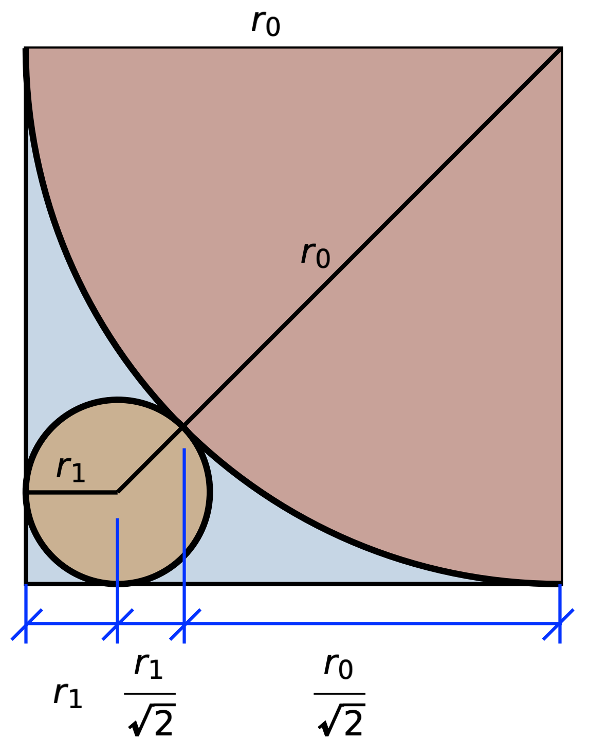
Don’t be offended—I trust you all to know why the horizontal components of the two diagonals are and . What I thought you might be questioning was my use of short diagonal ticks instead of arrowheads on the dimension lines along the bottom of the drawing.
This is a style I picked up as an undergrad. I use it all the time in hand-drawn sketches, and I think I’m going to use it here from now on. The first person I saw using this kind of dimension line was John Haltiwanger, who taught the second structural analysis class I took, and I adopted it in emulation of him. I mentioned Prof. Haltiwanger and his insistence on good sketches in this post last year.
There are two advantages to using ticks instead of arrowheads: speed and clarity. The speed advantage is obvious. Clarity comes in drawings of structural problems, where we use arrowheads to represent forces. Although it’s usually clear from context which lines are for forces and which are for dimensions, sometimes the two cross or are close enough to one another that it helps to use different ends. This is especially true when sketching on paper or a blackboard, where you can’t use line thickness to distinguish between the two.
Let’s say I’m going to analyze a simply supported beam with a uniformly distributed load across its entire length and a concentrated load at its center. I’d sketch it this way in my notebook:
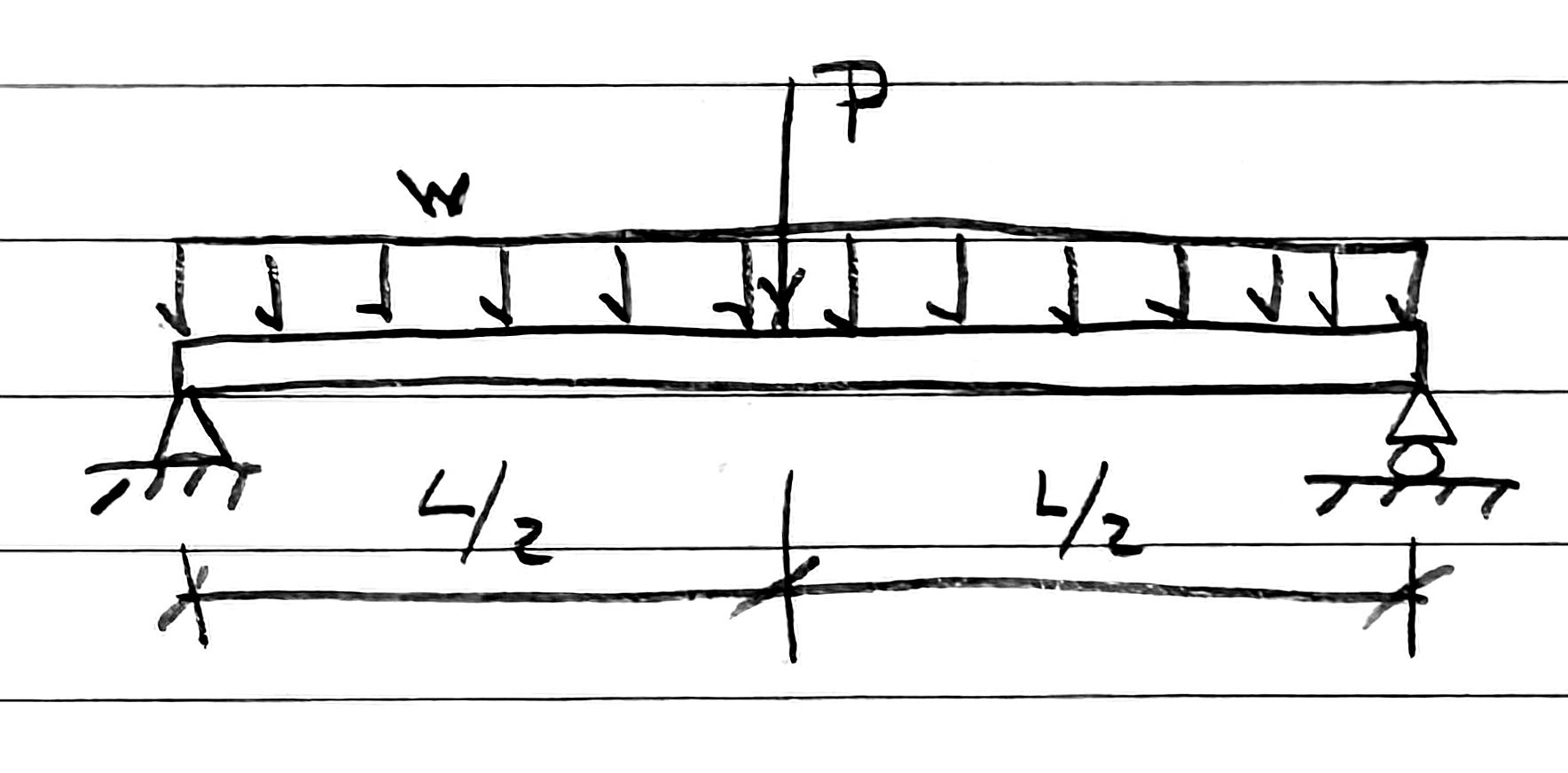
After drawing the beam, supports, and forces, I make the vertical leader lines, one long dimension line the full length of the beam, and then three quick diagonal ticks.
If I’m going to blog about it, I’ll turn it into a nicer drawing in OmniGraffle:

Using blue for the leader and dimension lines—and making them thinner—is a good way to distinguish them from forces, and I’ve been doing that for years.1 I’ve usually used a different style of arrowhead for the dimensions than for the forces. OmniGraffle has a huge number of arrowhead styles:
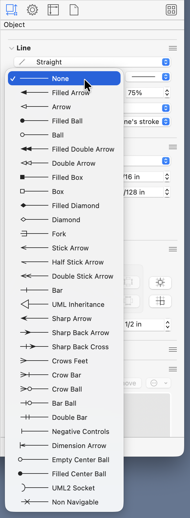
I’ve generally used the “Filled Arrow” for forces and the “Sharp Arrow” for dimensions. You might think I’d use the “Dimension Arrow,” but I’ve never liked it. It has a little leader line attached to it, which is, unfortunately, pretty much useless because it’s always the same length. Leader lines are supposed to draw your eye from the object to the dimension line—they have to be different lengths, and they’re usually much longer than the tiny ticks OmniGraffle provides.
I could continue to use the sharp arrows, of course, but I’ve decided my drawings here should look more like the sketches I make in my notebook. And it’s a nice tribute to Prof. Haltiwanger. Although his was my second structural analysis class, it was the one in which I began to truly appreciate the topic.
While I’m at it, I should mention that I made a set of stencils with objects commonly seen in structural analysis drawings.

The top two rows show fixed, simple, and guided ends; the bottom two rows show springs. There are four variations on simple ends; the differences depend on whether there’s a roller and whether I want to show the hinge explicitly. There’s only one linear spring, but I needed four rotational springs to account for different angles of attachment. All of these can be rotated as needed once they’re placed in an OmniGraffle document.
-
As you can see, I have not been consistent in my use of blue or black for the dimensions themselves. ↩
Easy to be hard
February 19, 2026 at 6:25 PM by Dr. Drang
Here’s a geometry puzzle from the March issue of Scientific American. If you see the trick, it’s easy to solve.1 After doing it the easy way, I decided to solve it again the hard way, as if I hadn’t noticed the trick.
Here’s the puzzle:
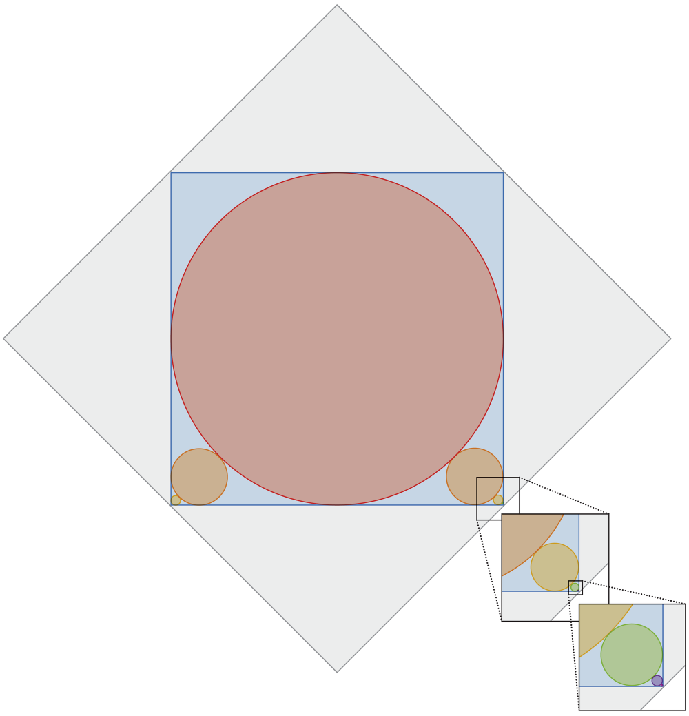
A red circle is inscribed inside a blue square. The arrangement leaves gaps in the square’s four corners, two of which are filled with smaller circles that just barely touch the big red circle and the two corner sides of the blue square. This, in turn, leaves two smaller gaps in the corners, which are filled with smaller circles, and so on, with ever smaller circles ad infinitum. The entire diagram is inscribed inside of a 1 × 1 gray square. What is the total circumference of all the circles?
Without the trick, we’re going to have to work out all the circumferences and add them together. We’ll start by figuring out the relationship between the radii of consecutive circles. Here’s a quarter of the largest circle, the radius of which we’ll call , and the next largest circle, the radius of which we’ll call :

From this drawing, we can express the width in two ways and set them equal to one another:
Multiplying through by and rearranging, we get
I want to turn this into a fraction with a 1 in the numerator, so I’ll multiply the top and bottom by an expression that will eliminate the square root in the numerator:
This relationship also holds for any two consecutive circles,
which means we can express the radius of the ith circle in terms of the radius of the largest circle:
So the sum of all the circumferences is times the sum of all the radii:
Note that there’s only one circle with radius , but two circles for all the other radii.
By the way, this expression is where it’s helpful to have the fraction inside the sum written with a 1 in the numerator. We know that
converges, so our fraction, which has a larger denominator, must also converge.
We’re nearly there. Recall that the gray square (the one that’s rotated 45°) has a side length of 1. That means
so the sum of the circumferences is
Now for a confession: I have always stunk at working out infinite series. Luckily, I can now lean on a computational cane. Here’s a Mathematica expression that will return the infinite sum:
Pi/Sqrt[2] (1 + 2 Sum[1/(3 + 2 Sqrt[2])^i, {i, 1, Infinity}])
The answer, as we know from doing it the easy way, is .
If I didn’t have Mathematica, I’d probably set up a finite series for the expression without ,
and run out the calculations for different values of n to see where it converges. We can show the results as a table,
| n | Sum |
|---|---|
| 1 | 0.94974747 |
| 2 | 0.99137803 |
| 3 | 0.99852070 |
| 4 | 0.99974619 |
| 5 | 0.99995645 |
| 6 | 0.99999253 |
| 7 | 0.99999872 |
| 8 | 0.99999978 |
| 9 | 0.99999996 |
| 10 | 0.99999999 |
or as a plot,
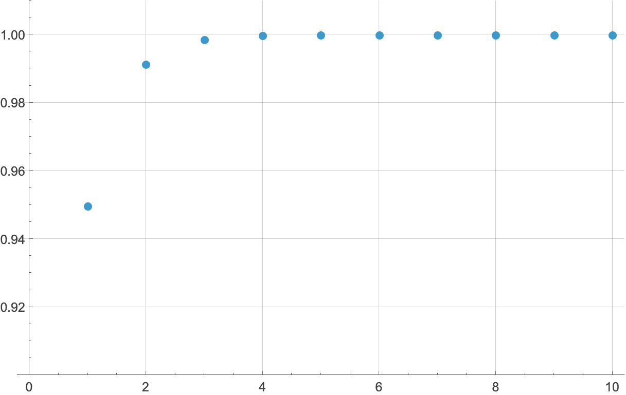
Either way, going out ten terms is overkill—it’s obvious that the sum is converging to 1, which means the circumference sum is converging to . You can, I guess, consider this numerical exercise as a check on Mathematica’s work. Or a check on the easy solution.
-
SciAm also uses the trick in its solution, which you won’t see if you click on the link in this paragraph. It’s one link further away. ↩
