Weekdays of future passed
May 2, 2024 at 10:01 PM by Dr. Drang
Some time ago, I wrote a little shell script called next, which used the date command to output the date some number of weekdays after the current date. So if I ran it today (Thursday, May 2, 2024) with this invocation,
next tue
it would return
2024-05-07
which is the Tuesday of next week. If I ran it with this invocation,
next tue 2
it would return
2024-05-14
which is the Tuesday after that, i.e., two Tuesdays after today.
This worked out pretty well, except that I had to run it in the Terminal1 and then copy the output if I wanted it to go into some document. The switching to the Terminal and back made next a lot less convenient than it should have been.
So I rewrote it as a Keyboard Maestro macro that I can run from anywhere and get the output onto the clipboard immediately. I call the macro , and you can download it (you may need to right-click on that link).
When is invoked, typically by ⌃⌘W, this window appears:

You choose the day of the week from the popup menu (the default is Monday) and enter the number of those weekdays after today in the text field (the default is 1).
Assuming I choose two Tuesdays from today, as in the second next example above, the output is this:

As you can see, it tells me what the date is and gives me the option to put it on the clipboard in either of two formats:
yyyy-mm-dd, which is what I’d typically use if I were making notes for myself.- Month Day, Year, which is what I’d use in an email or text to someone else (probably deleting the year).
Or I can just the macro if all I want is to see the date.
Because has more options than next, it’s more complicated, but it still uses date to do most of the work. Here’s the code:

The key is the shell script in the second step:
weeks=$(( $KMVAR_Local_Number - 1 ))
date -v+${weeks}w -v+1d -v+$KMVAR_Local_Chosen_Weekday '+%Y-%m-%d'
The first line subtracts 1 from the number of weekdays the user asks for and puts that into the variable $weeks. The second line does the work. The first two -v options tell date to move forward $weeks weeks and one day. The third -v option tells it to move to the weekday chosen by the user. The final argument is the output format.
If I asked for the second Tuesday after today, as in the example, date would be called like this:
date -v+1w -v+1d -v+Tuesday '+%Y-%m-%d'
which returns 2024-05-14. The -v option is pretty complicated, and I frankly don’t trust myself to give you a complete explanation of how it works. I suggest you RTFM and play around with it, possibly using the command above as your starting point.
OK, so that’s where we get the yyyy-mm-dd form of the date. It’s stored in the Local Next Weekday variable. The next shell script converts it to the long format through
date -jf '%Y-%m-%d' $KMVAR_Local_Next_Weekday +'%B %-e, %Y'
The -jf combination of options is the common way to convert dates from one format to another. The -f part has an argument that specifies the input format, and the -j part says that the input date should not be used to set the computer’s date and time.
Yes, date can be used to set the date, which sounds insane, but only the superuser can do that. Option letters usually have some relationship to what they do, but -j has always seemed to me like a weird choice to turn off the date-setting feature. I’ve decided it stands for Jesus, don’t try to change the date!
The third script in the macro is a Python script to turn the cardinal number (1, 2, 3, etc.) stored in Local Number into the ordinal number (1st, 2nd, 3rd, etc.) that’s used in the prompt of output window. This is an unnecessary bit of flair that I added to the macro because I already had the code to do it.
python:
#!/usr/bin/env python

import os

n = int(os.environ['KMVAR_Local_Number'])

s = ('th', 'st', 'nd', 'rd') + ('th',)*10
v = n%100
if v > 13:
  print(f'{n}{s[v%10]}')
else:
  print(f'{n}{s[v]}')
The last two steps of the macro are pretty straightforward. They display the output window and handle whatever button the user presses.
One last thing. If you think I misspelled “past” in the title of this post, you need to clear the X-Men out of your head. There’s a reason the examples get the dates of Tuesday afternoons.
Over center
May 1, 2024 at 1:48 PM by Dr. Drang
I saw Steve Mould’s latest video this morning. It’s about mechanisms that store elastic energy and release it quickly. His examples come from insects and human-made devices. You should take 15 minutes and watch it.
In previous reviews of Mould’s videos (here and here), I did some mechanics analysis to explain the videos in a more detailed (or just plain different) way. I’m not going to do that today, but I do have a brief comment on the question he raises at the end of the video, starting at about the 11:30 mark.
It concerns this mechanism he made with two rods hinged together and connected at their far ends by an elastic band.
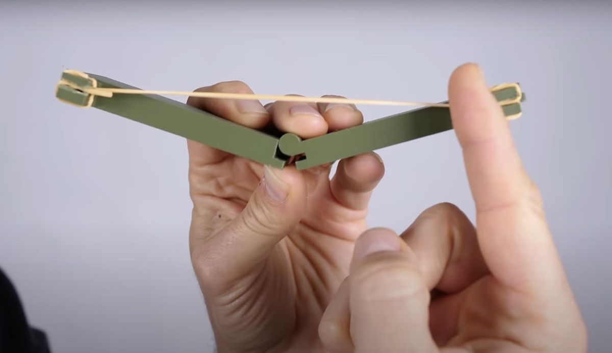
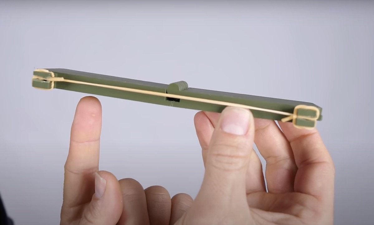
Here’s his description:
It gets harder and harder to open this thing up as the elastic becomes more and more stretched. But actually, beyond a certain point it gets easier again. And that’s because of the shallow angle of the elastic. Only a small component of the force from the elastic is perpendicular to the arm. So it gets easier and easier and easier until it passes the pivot point. It’s actually slightly holding it open now. And you only need a really small force to close it again.
Mould felt sure he’d seen this kind of mechanism before, but he couldn’t come up with an example. He asked around and didn’t get any satisfactory answers, probably because he was asking a bunch of physicists and mathematicians.
It’s an over-center mechanism. I can’t think of any engineer or mechanic I’ve ever known who wouldn’t identify it immediately as such. It’s commonly used to latch or lock mechanisms in place. The most obvious example I could get my hands on in a hurry was a pair of vise grips.
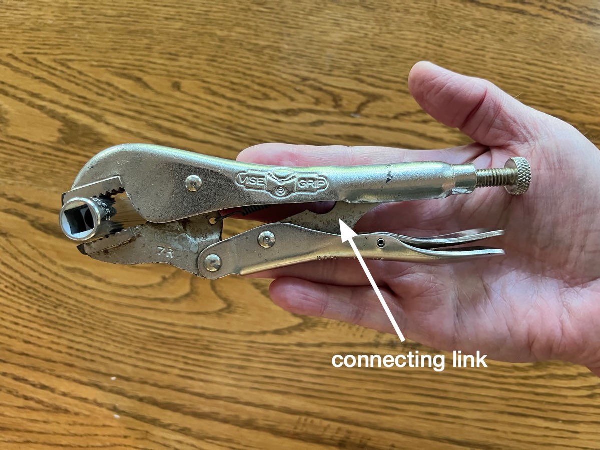
As you squeeze the handles together, the mechanism reaches a point where the connecting link that runs between the handles snaps through into the locking position and whatever is between the jaws is held securely with no more effort from the user.
Another example is the latch on my toolbox.1
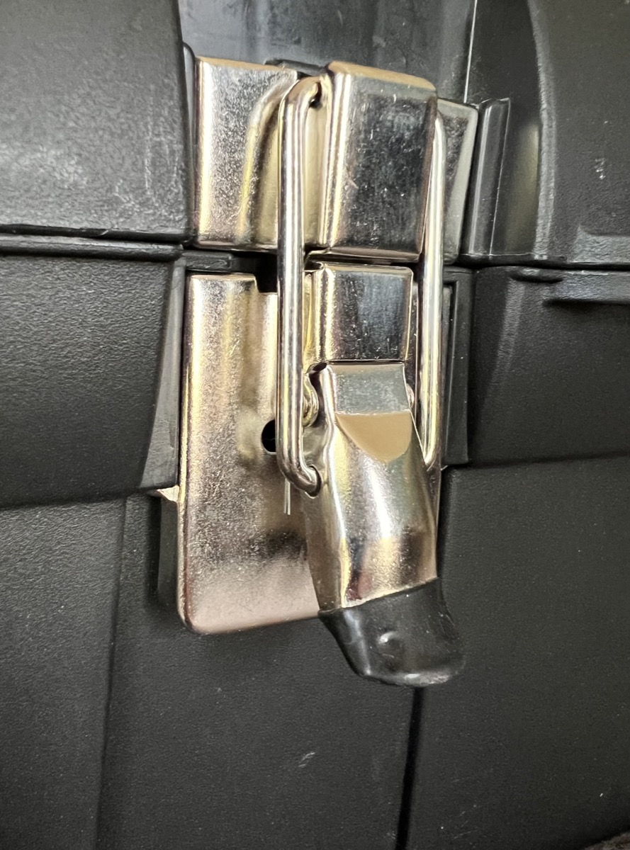
Here it’s in the not-quite-latched position. When you push the bottom end of the lever the rest of the way in, the inverted U of the clasp squeezes the parts together and moves to the other side of the lever’s pivot point, locking the mechanism in place.
What’s interesting about Mould’s attempts to describe the mechanism is that he very nearly comes up with its name. He says “over the hump” a couple of times, and that is so close to “over center” that I half-expected him to answer the question on his own before the end of the video.
“Over the hump” reminds me of this post (one of my favorites) about the load-deflection curve of a toggle mechanism. Which is also an over-center device.
-
Why didn’t I notice the latch on the toolbox before I opened it to pull out the vise grips? Because I had vise grips on my mind. ↩
Building Newmark’s influence chart
April 26, 2024 at 2:03 PM by Dr. Drang
After writing the last post, I decided to do the calculations necessary to make Newmark’s influence chart.
I started with the Boussinesq equation:
If you compare this with the formula I gave last time, you’ll see that I’ve deleted the negative sign. That’s because tensile stresses seldom arise in soil mechanics, so the convention is to take compressive stresses as positive.
This is a solution to the elasticity equations in cylindrical coordinates, , where the origin of the coordinate system is at the point on the surface where the load is applied. Notice that there’s a circular symmetry to the solution— is independent of the angle .
This symmetry has an interesting and very useful consequence. We can move the origin of the coordinate system to the point on the surface above the point at which we are calculating the stress, and the formula for will remain the same. We’ll use this to figure out the stress1 associated with a distributed load.
Because Newmark has made his chart as a series of rings split into sectors, we’re going to calculate the stress due to a uniform distributed load, , acting over one of these sectors. The two radii that bound the sector are and , and the two angles that bound the sector are and .
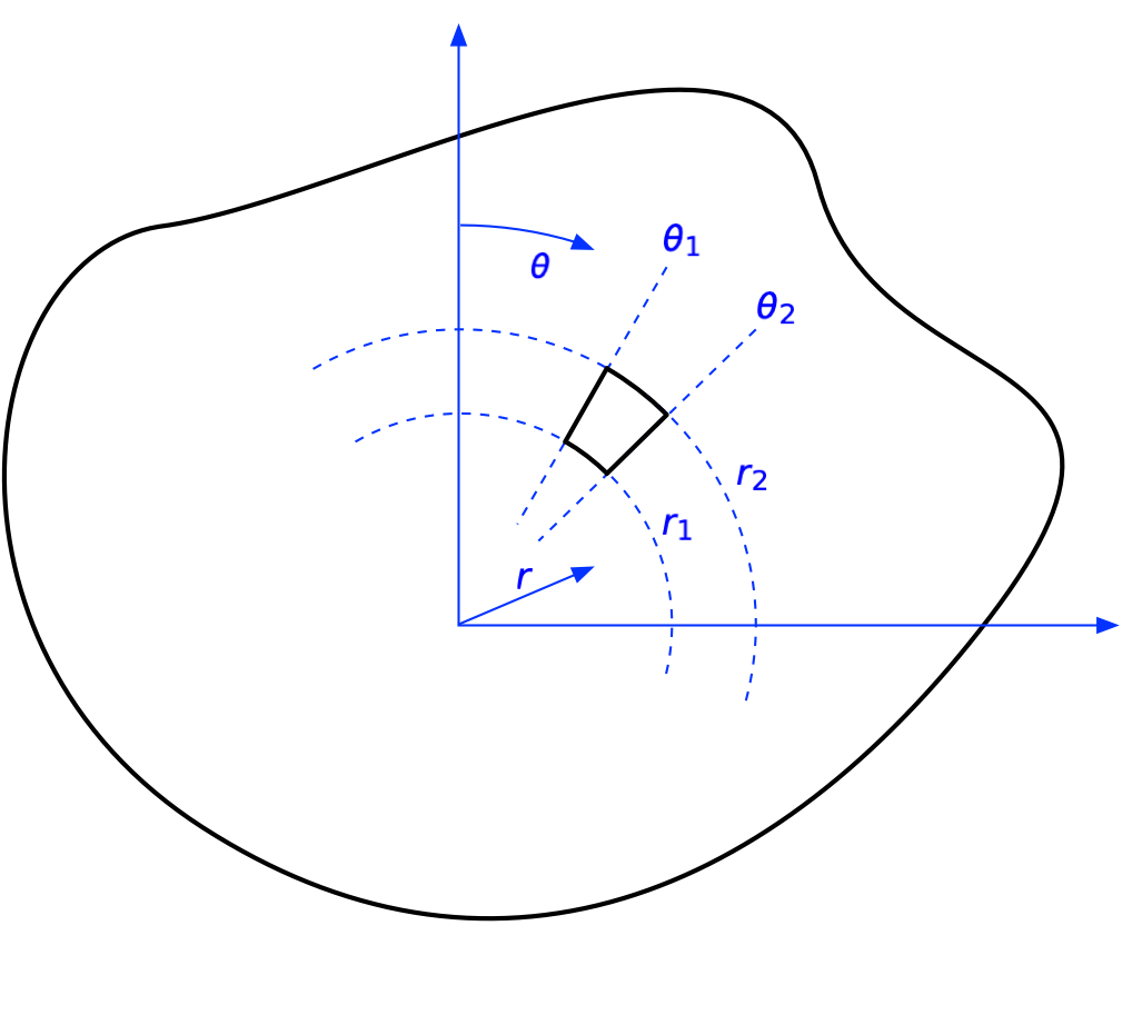 With this loaded area defined, we can write the resulting stress as
Because the integrand doesn’t contain , that part of the integral will result in a term, which we’ll call . That term, along with the constants, can be brought outside the integral over :
If there were an analytical solution to this integral, we’d be in business, but I don’t think there is. I gave the problem to Mathematica, and it thought for over five minutes without coming up with an answer before I stopped it. So we’re going to have to use numerical integration, which means it’s time to nondimensionalize the equation.
First, we note that is nondimensional. This fits in with Newmark’s scheme, because this is what he calls the influence value (see the lower right corner of the chart). So we know this term is going to be 0.001.
Second, we see that Newmark split each ring into an integral number of sectors. The number of sectors isn’t the same for each ring, but we can always say that
where is a positive integer. Therefore,
Finally, we note that Newmark scales the radii of the rings by the depth, . So we’ll define a new variable, , and rewrite the integral using this change of variable. We see that
and (this may not be as obvious, but you can check it)
So with these substitutions, we get
Hey, look! The ’s all cancel out, and we’re left with
Note that all the terms in this equation are pure numbers; none of them have any units, like feet or meters or pounds. That’s what I meant by “nondimensionalize.”
So now all we have to do is find a sequence of values for and that will solve this equation for the appropriate value of . Starting at the origin of the chart, we know that and (you may have to zoom in to see that), and we can solve for . Then for the next ring, we use the previously calculated value of as our new value for and set . This continues on for all 25 rings in the chart.
The box below should contain the Mathematica notebook I used to do the calculations. If it’s empty, that means the Wolfram Cloud is being slow and stubborn, so you might have better luck following this link. Or not. I don’t have a lot of experience with the Wolfram Cloud, but so far I’ve noticed that it isn’t as responsive as the documentation would have you believe.
Whether you have any experience with Mathematica or not, I think the logic of the notebook is relatively easy to follow. For each pass through the Do loop, we’re calculating a new upper limit for the numerical integral that solves the equation. That value is then appended to the list of radii and gets used as the lower limit of the numerical integration during the next loop. Finally, the ring thicknesses are calculated by subtraction.
The results are summarized in this table:
| Ring | Sectors | Outer radius | Thickness |
|---|---|---|---|
| 1 | 8 | 0.07327 | 0.07327 |
| 2 | 16 | 0.12778 | 0.05450 |
| 3 | 24 | 0.18259 | 0.05481 |
| 4 | 24 | 0.22600 | 0.04342 |
| 5 | 24 | 0.26382 | 0.03781 |
| 6 | 48 | 0.33048 | 0.06667 |
| 7 | 48 | 0.39080 | 0.06032 |
| 8 | 48 | 0.44807 | 0.05727 |
| 9 | 48 | 0.50413 | 0.05606 |
| 10 | 48 | 0.56025 | 0.05612 |
| 11 | 48 | 0.61747 | 0.05723 |
| 12 | 48 | 0.67678 | 0.05931 |
| 13 | 48 | 0.73921 | 0.06243 |
| 14 | 48 | 0.80596 | 0.06675 |
| 15 | 48 | 0.87854 | 0.07258 |
| 16 | 48 | 0.95895 | 0.08041 |
| 17 | 48 | 1.05003 | 0.09108 |
| 18 | 48 | 1.15606 | 0.10603 |
| 19 | 48 | 1.28396 | 0.12790 |
| 20 | 48 | 1.44608 | 0.16213 |
| 21 | 48 | 1.66772 | 0.22164 |
| 22 | 48 | 2.01358 | 0.34586 |
| 23 | 32 | 2.41493 | 0.40135 |
| 24 | 32 | 3.31945 | 0.90452 |
| 25 | 16 | 4.89898 | 1.57953 |
The inner radius of each ring is the outer radius of the ring before it. The exception is the first ring; recall that its inner radius is zero.
My first thought after running out these calculations was to check the numbers against measurements I could take from the chart. They were pretty close. Not perfect, but typically within a couple of percent. I couldn’t really expect any better, as the chart (which is a page from this PDF) wasn’t scanned at a particularly high resolution (only 150 dpi), and it wasn’t perfectly aligned with the scanner (the horizontal axis isn’t quite horizontal).
But would Newmark include a chart without giving the data necessary for readers to reproduce it? Of course not. In the appendix is a table of values for making all the various influence charts discussed in the paper.2 Here’s an excerpt from the table that shows the ring radii for the vertical pressure influence chart.
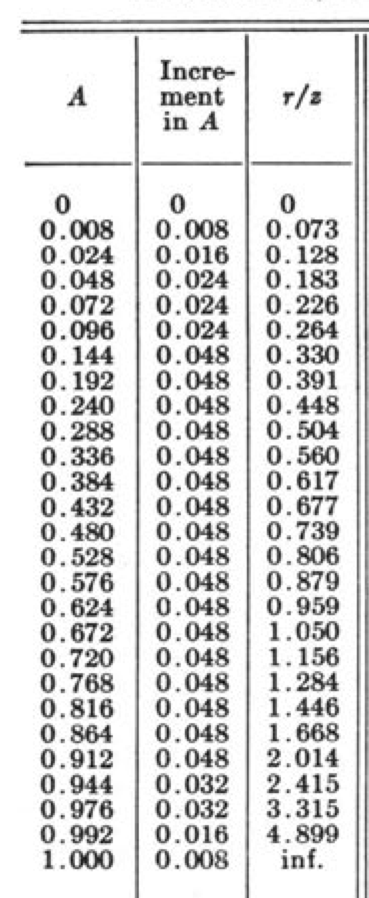
It’s the third column, which gives the radius as a fraction of the depth, , that we can compare to the “Outer radius” column in the table above. As you can see, all the numbers match to three decimal places except the one for the 24th ring. Newmark shows 3.315, when the value should be 3.319. Should we blame the student who did the calculations, noted in the acknowledgments as Harold Crate? Should we blame the unacknowledged secretary who typed up Crate’s calculations? No, we have to blame Nate Newmark himself—after all, he’s the guy whose name is mentioned in all the soil mechanics textbooks.
-
If you haven’t noticed yet, I’m using the words, stress and pressure interchangeably because for this problem they are the same when I’m talking about what’s going on at depth in the soil. ↩
-
I’ve only discussed the chart for vertical pressure, but Newmark also provides charts for shear stresses, maximum principal stress, and so on. ↩
Boussinesq and Newmark
April 25, 2024 at 1:31 PM by Dr. Drang
In a post this morning, John D. Cook listed several types of partial differential equation that are unusual in that they can be solved analytically. The last one in his list caught my eye because it’s one that I know pretty well from the theory of elasticity: Boussinesq’s equation.
Consider a linearly elastic body with a planar boundary that is infinite in extent below that boundary. Now apply a point load normal to the plane on that boundary:
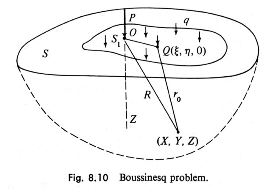
Figure from Introduction to the Mechanics of a Continuous Medium by Lawrence Malvern
The solution for the vertical stress, , at a depth and a horizontal distance from the point of application of load is
This solution was derived by Joseph Boussinesq in 1885. Geotechnical engineers later found this solution interesting because it gave them an opportunity to calculate subsurface pressures in soil due to the weight of a building founded on that soil. It isn’t perfect because soils aren’t linearly elastic, but it’s a reasonable approach to making estimates, which is what engineering is all about.
Now, the Boussinesq equation is for a point load, and buildings aren’t points—buildings distribute their weight over their foundation footprint. In theory, this isn’t a problem, because we can handle the distributed load by integration. In practice, it’s a pain in the ass, because the integration has to be done numerically for realistic building footprints and, furthermore, has to be done repeatedly for different depths and different locations under the building. A nonstarter in the pre-computer era.
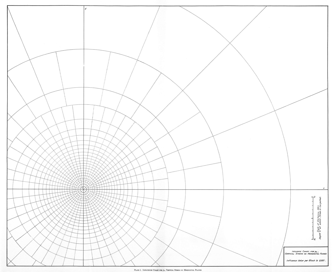
In 1938, Nathan Newmark, then a young professor in the Department of Civil Engineeering at the University of Illinois (my alma mater), came up with a graphical solution to the integration problem. He devised an influence chart that looked like this:

Figure from Engineering Experiment Station Bulletin No. 338
Here’s a more readable view of the scale and other information in the bottom right corner:
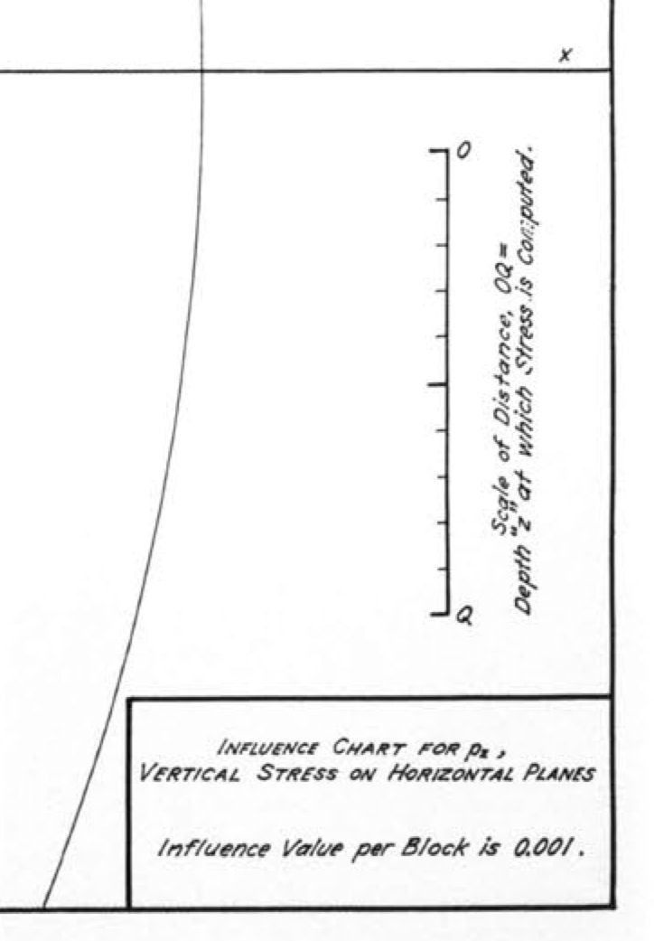
To figure out the vertical pressure in the soil at a given depth, you take that depth to be the distance OQ shown above and draw an outline of the foundation plan to that scale on tracing paper. You then put the drawing on the influence chart and position it so that the horizontal position at which you want the soil pressure is at the center of the chart. For example, if our building plan is a fat ell shape, 50′×75′ with a 25′×25′ chunk taken out of the southwest corner, and we want to calculate the soil pressure under the inside corner at a depth of 25′, we take OQ to be 25′, draw an outline of the building to that scale, and place the drawing with the inside corner at the center of the concentric circles. Like this:
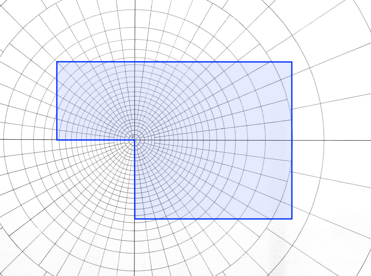
Now we count the number of “squares” the building covers and multiply that by two values:
- The average pressure of the building (its weight divided by the area of its footprint).
- The chart’s influence value of 0.001, which is given in the lower right corner of the chart.
The result is the soil pressure 25′ below the inside corner. To get the pressure at other horizontal positions, we slide the drawing around and count the squares again. To get the pressures at another depth, we redraw the building footprint at a scale appropriate for that depth.1
I’m not saying there isn’t a degree of tedium to this, but it’s a hell of a lot easier than doing multiple numerical integrations on paper with a slide rule and a desk calculator.
The soil pressure influence chart was hardly Newmark’s only contribution to engineering. He was a genius at coming up with alternate ways of seeing problems and devising solution techniques that could be used by everyday engineers working in design offices. Many of these techniques have been superseded by computer-based methods, but at least one—the beta method for structural dynamics problems—is still going strong.
Newmark had moved to emeritus status by the time I was a student; he died during my senior year. The department shut down for a day so the faculty could attend his funeral. Not only had he been their colleague, for many he had been their thesis advisor. This group included my advisor; academically, I am one of Newmark’s many grandchildren.
-
There’s also a pressure component due to the weight of the soil itself, but that’s just the unit weight of the soil multiplied by the depth. Add that to the value calculated via the influence chart to get the total vertical pressure in the soil. ↩

